From TakeOut to TakeIn: The Savings Simulator
By Ken Koon Wong in r R simulation saving pert motivation
August 13, 2023
Saving can be enjoyable! If you’re planning to cut down on takeout orders, why not use past data to simulate your savings? Let it inspire and motivate your future dining-in decisions! 👍

If you’re anything like me, you might often resort to takeout due to the convenience of app-based orders and deliveries. These expenses can pile up quickly, especially if you’re ordering 2 or 3 times a week. So, how can we motivate ourselves to cut back on takeout and perhaps track our potential savings as an incentive?
Disclaimer:
This won’t literally add money 💰 to your bank account. Instead, it simulates your past spending to show what you might have spent on takeout today had you not cut back 🤣. It’s all for motivation. Think of the ‘money saved’ feature as a hypothetical tally.
Thought process:
- Generate a distribution of your expenditures and save the data.
- Set up a script to run daily, sample from this distribution, and store the results.
- Receive motivational emails!
Generate a distribution of your expenditures and save the data.📊
One can easily download credit card data from their bank and use it as a sample from the prior year, assuming current takeout habits remain unchanged and prices haven’t shifted significantly. This is perhaps the simplest method.
However, one can also sample from a chosen distribution to replicate these spending habits. For illustrative purposes, let’s exaggerate a bit: assume we order four times a week with a per-order cost ranging from $50 (minimum) to $200 (maximum), with a mode cost around $80.
PERT Distribution
There’s a particular distribution I’ve been keen to explore – the PERT distribution. While I’m not entirely sure of its suitability here, it’s worth an experiment. The PERT distribution is frequently employed in project management, risk, and decision analysis, especially when modeling activity durations. Some of its merits include flexibility, intuitiveness, and its capacity to account for uncertainty. It becomes especially valuable when historical data is scarce, and experts need to rely on judgment to estimate certain parameters. With the PERT distribution, they can encapsulate their uncertainty in a structured tri-point format. To learn more, visit here
Let’s code!
library(freedom)
library(tidyverse)
library(lubridate)

# 4 times takeout per week, calc how many days per year
n <- 4*52
min <- 50
mode <- 80
max <- 200

# sampling from modified PERT distribution
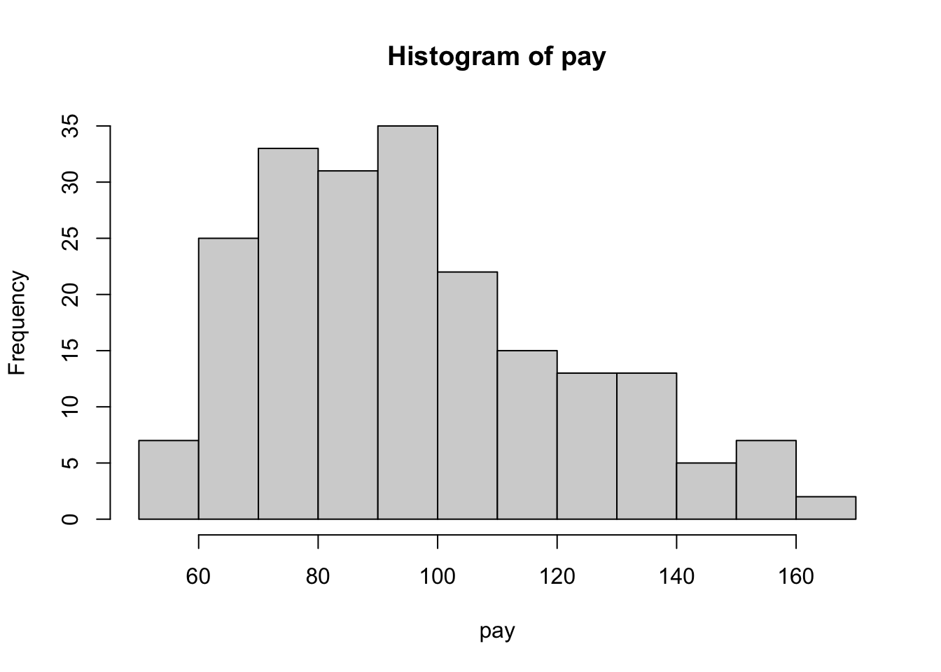
pay <- rpert(n = n, x.min = min, x.max = max, x.mode = mode, lambda = 4)

# visualize pay
hist(pay)

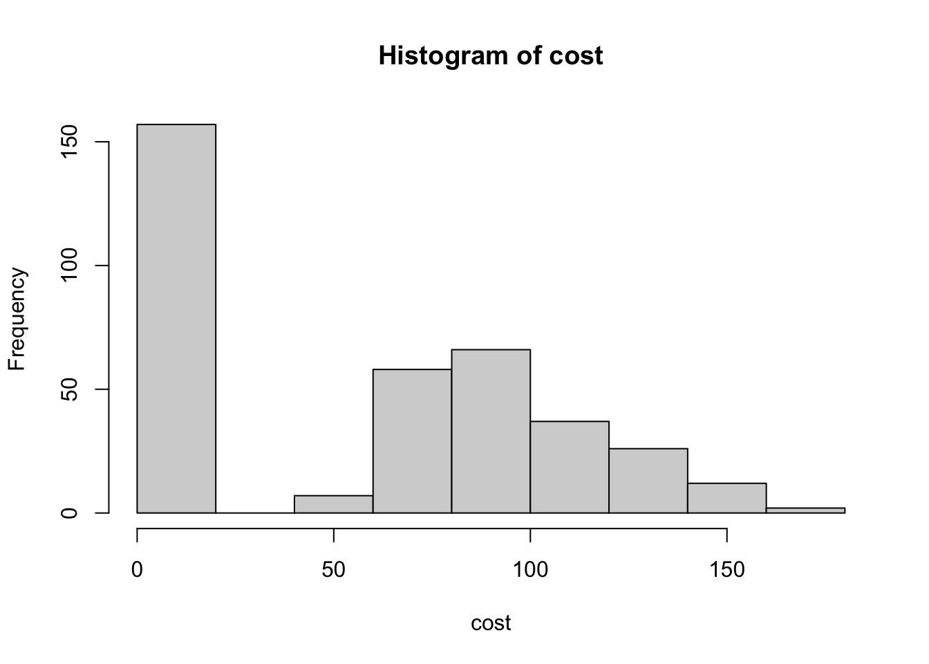
# making zeros for days did not take out
nopay <- rep(0, 365-n)

# combine both
cost <- c(pay,nopay)

# visualize cost
hist(cost)

# simulate for 28 days
sample(cost, 28, replace = T)
##  [1]   0.00000   0.00000  90.05571  68.38042 111.59603   0.00000  98.65783
##  [8] 111.74102  68.02683 106.28409   0.00000 132.80770 124.57875   0.00000
## [15] 131.47773 106.33280  98.25207 128.52828   0.00000  67.02519   0.00000
## [22] 126.47210   0.00000  75.70615   0.00000   0.00000  60.63034  72.27573
# save(cost, file = "cost.rda") # only need to do these once

# create a csv that has the first data
df <- tibble(date=mdy("8/12/23"), day=1, total=0)

# write_csv(df, file = "data.csv")
Perfect! Make sure to save the distribution so we’re not simulating that every time we run the script.
Set up a script to run daily, sample from this distribution, and store the results. 🤖
# load the prior cost distribution for the entire year
load(file = "cost.rda")

# load data csv
df <- read_csv("data.csv")

# run simulation for today
date <- Sys.Date()
diff_day <- ymd(date) - ymd(df[[1,1]])
day <- df[[1,2]] + diff_day[[1]]
total <- sample(cost,1)

# update our df
df <- df %>%
  add_row(date=date,day=day,total=total)

# how much total have we saved?
total_saved <- df %>%
  pull(total) %>%
  sum()

# how much we saved today?
last_saved <- df %>%
  tail(1) %>%
  pull(total)
Receive motivational emails! 📧
# send email via your preferred email server, here we use gmail
from <- Sys.getenv("auto_email") # get your robot user acct from R environment
to <- c("savebydiningin@gmail.com","simulateyoursaving@gmail.com")
message <- paste("Subject: Total saved: $",total_saved,"\r\n\r\n",paste0("Today, for not ordering from take out delivery, you saved $",last_saved, ". And so far you saved a total of $",total_saved),collapse = "\r\n")

# # in case your want to send to multiple people one at a time instead of group email
for (i in to) {

  send_mail(mail_from = from,mail_rcpt = i, smtp_server = "smtps://smtp.gmail.com:465", message = message,verbose = TRUE, username = Sys.getenv("auto_email_user"), password = Sys.getenv("auto_email_pass"))
  Sys.sleep(15)
}

# save the new data
write_csv(df, path = "data.csv")
The email looks like this

Hypothetically, how much did we save if we dine in for 28 days with the distribution above?
save_a_month <- sample(cost, 28, replace=T)
save_a_month
##  [1]   0.00000  84.15510   0.00000  84.15510 101.64545   0.00000  96.02335
##  [8]   0.00000  94.23887   0.00000  91.25703   0.00000 166.20857 112.62427
## [15]   0.00000   0.00000   0.00000   0.00000  77.28963  72.38574   0.00000
## [22] 139.16093  82.51321 120.83317  60.19978   0.00000   0.00000  71.10075
Wow, we saved 1453.7909519 !!! That’s some motivation that builds up everyday. Assuming we don’t get discouraged from the zeros 🤣
Improvements or other ideas:
- If you own a Raspberry Pi, you can configure crontab to execute the script at a specific time each day.
- One of the advantages of saving this data as a CSV is its flexibility. If you did order takeout today, simply add a new row and insert
-80(or the respective amount spent) to deduct it from the savings. - If there’s a specific item you’re hoping to purchase, you can set a price threshold. Once your savings reach this amount, an email notification can be triggered.
- Visualize your spending habits before and after the intervention to discern the difference. For a more in-depth analysis, consider employing the ‘difference-in-differences’ econometric technique.
Happy Saving!

Lessons learnt
- The PERT distribution is intriguing. Its flexibility may be just what I need, especially when considering clinical judgment for prior distribution.
- Coding can be both enjoyable and advantageous. In situations like this, it sparks motivation to save—albeit in a hypothetical manner. The only limit is imagination!
If you like this article:
- please feel free to send me a comment or visit my other blogs
- please feel free to follow me on twitter, GitHub or Mastodon
- if you would like collaborate please feel free to contact me
- Posted on:
- August 13, 2023
- Length:
- 5 minute read, 1025 words
- Categories:
- r R simulation saving pert motivation
- Tags:
- r R simulation saving pert motivation