Learning & Exploring Survival Analysis Part 1 - A Note To Myself
By Ken Koon Wong in r R survival analysis time-to-event analysis survival function hazard ratio simulation
May 2, 2026
A note to myself on survival analysis — KM curves, log-rank tests & Cox models 🧮 If I wrote it the way I understood it, maybe I’ll actually remember it 🤞
Motivations
We see survival analysis or more generally called time-to-event analysis almost all the time when we review journals articles on NEJM etc. Even though we understand the heuristic in interpreting some of the simpler result, I realized that I need to look at this a bit closer to full understand the works and math behind it. There was a recent project that made me feel that my understanding of this is not as competent as I had hoped after talking to one of my statistician colleagues, who also so happen to wrote this blog. Please take a look at Emily’s blog for a better, and a more accurate survival analysis tutorial. This blog is more for my learning so that I can refer back the fundamental when I need a refresher in the future. Also, if I were to write it the way I understood it, maybe that might increase the probably of me recollecting what I understood before. What are we waiting for? Let’s time-to-event this analysis!
Objectives:
- Survival function
- Let’s Calculate By Hand
- Simulation
- Acknowledgement
- Oppotunities For Improvement
- Lessons Learnt
Time-to-event Analysis
The name “survival analysis” is a bit misleading if you first encounter it outside of clinical research. The “survival” doesn’t necessarily mean staying alive — it means surviving without experiencing the event. But that even does not necessarily have to be mortality. It could be an unwanted event etc. Outside of clinical research, an event could be the time when a waymo arrives at your doorstep or someone flaked out. 🤣 Hence time-to-event analysis appears to be more a better terminology, in my opinion.
This is different from the good ol regression is because time is the outcome, not only that it occurred or not (binary), but when! Now then if you’re like me, that’s just negative binomial regression, right? Not quite. Because, there is an additional special feature to time-to-event analysis called censoring.
Censoring can mean that the event did not occur, but it can also mean that we lost track of the patient, or the study ended before the event occurred.
I don’t know about you. But for me, censoring has a negative connotation. It sounds like we’re hiding something. But in survival analysis, censoring is actually a good thing. It means we have partial information about the time to event, even if we don’t know the exact time. So, think of censoring as the last time we noticed that the event DID NOT happen, and it’s usually coded as 0. In good ol regression, we usually will either do a complete case analysis (throw out missing data) or impute. But, imputing outcome is a tad odd,
in most cases except here. The common censoring is right censoring, meaning we lose track of someone on the right side of the timeline.
Survival Function
The survival function, written S(t), answers one simple question: “What is the probability that a person has NOT yet experienced the event by time t?”. At t=0, everyone is event-free, so S(0) = 1 (100%). As time goes on, people experience the event, and S(t) decreases.
Let’s Calculate By Hand
| patient | time (months) | status |
|---|---|---|
| A | 2 | 1 (event) |
| B | 3 | 0 (censored) |
| C | 5 | 1 (event) |
| D | 6 | 1 (event) |
| E | 8 | 0 (censored) |
Alright, the above looks quite self-explanatory. We have 5 patients, and we are tracking their time to event in months. Patient A experienced the event at 2 months, while patient B was censored at 3 months (we lost track of them). Patient C had the event at 5 months, patient D at 6 months, and patient E was censored at 8 months. Now let’s do some calculation.
Formula: $$ \hat{S}(t) = \prod_{i:, t_i \leq t} \left(1 - \frac{d_i}{n_i}\right) $$
\(\hat{S}(t)\): The estimated survival function; the probability of surviving beyond time\(t\).\(\prod_{i:\, t_i \leq t}\): Product over all event times\(t_i\)that are less than or equal to\(t\).\(t_i\): The\(i\)-th observed event (death/failure) time.\(d_i\): The number of events (deaths/failures) that occurred at time\(t_i\).\(n_i\): The number of individuals at risk (still alive and under observation) just before time\(t_i\).\(\frac{d_i}{n_i}\): The estimated probability of the event occurring at time\(t_i\).\(1 - \frac{d_i}{n_i}\): The estimated probability of surviving through time\(t_i\).
or simplistically:
\(S(t) = S(t-1).(1-d/n)\)
Let’s calculate by hand:
| time | at risk (n) | event (d) | S(t) |
|---|---|---|---|
| 0 | 5 | 0 | 1 |
| 2 | 5 | 1 | 1*(1-1/5)=0.8 |
| 3 | 5-1=4 | 0 | 0.8*(1-0)=0.8 |
| 5 | 4-1=3 | 1 | 0.8*(1-1/3)=0.5333 |
| 6 | 3-1=2 | 1 | 0.5333*(1-1/2)=0.2667 |
| 8 | 2-1=1 | 0 | 0.2667*(1-0)=0.2667 |
That’s interesting! I don’t think I’ve calcualte these by hand before and that’s very helpful in just doing a simple example and observing the result. Alright, when we read articles, there typically is a group factor, how do they then use KM to generate 2 survival curves or survival estimate for each group? They just do the same thing but only for the subset of the data that belongs to that group. So, if we have a treatment and control group, we would calculate S(t) separately for each group, and then we can compare the two survival curves to see if there is a difference in survival between the groups. How? We can use the log-rank test to compare the survival curves, or we can use a Cox proportional hazards model to estimate the hazard ratio between the groups. Now, things are starting to look a tad more familiar. Let’s use R and some simple example and see if we can get to log-rank test on just simple KM etimator.
library(tidyverse)

simple_df <- tribble(
  ~time, ~status, ~treatment,
  5,1,1,
  2,1,0,
  6,0,1,
  1,1,0,
  2,0,1,
  2,0,0,
  7,1,1,
  3,1,0,
  7,1,1,
  2,1,0,
  1,1,0,
  6,1,1
) |>
  mutate(subject = row_number())

treatment_df <- simple_df |>
  filter(treatment == 1) |>
  arrange(time)

treatment <- tibble()
time <- treatment_df |> distinct(time) |> pull()
at_risk <- nrow(treatment_df)
S_t <- 1

for (i in time) {
  df_i <- treatment_df |>
    filter(time == i)
  status <- df_i |> pull(status) |> sum()
  n <- df_i |> pull(status) |> length()
  S_t <- S_t * (1 - status/at_risk)
  treatment <- treatment |>
    bind_rows(tibble(time=i,at_risk=at_risk,S_t=S_t,treatment=1))
  at_risk <- at_risk - n
}

(treatment)
## # A tibble: 4 × 4
##    time at_risk   S_t treatment
##   <dbl>   <int> <dbl>     <dbl>
## 1     2       6   1           1
## 2     5       5   0.8         1
## 3     6       4   0.6         1
## 4     7       2   0           1
no_treatment_df <- simple_df |>
  filter(treatment == 0) |>
  arrange(time)

no_treatment <- tibble()
time <- no_treatment_df |> distinct(time) |> pull()
at_risk <- nrow(no_treatment_df)
S_t <- 1

for (i in time) {
  df_i <- no_treatment_df |>
    filter(time == i)
  status <- df_i |> pull(status) |> sum()
  n <- df_i |> pull(status) |> length()
  S_t <- S_t * (1 - status/at_risk)
  no_treatment <- no_treatment |>
    bind_rows(tibble(time=i,at_risk=at_risk,S_t=S_t,treatment=0))
  at_risk <- at_risk - n
}

(no_treatment)
## # A tibble: 3 × 4
##    time at_risk   S_t treatment
##   <dbl>   <int> <dbl>     <dbl>
## 1     1       6 0.667         0
## 2     2       4 0.333         0
## 3     3       1 0             0
Visualize
rbind(treatment,no_treatment) |>
  bind_rows(tibble(
    time=c(0,0), status=c(0,0), treatment=c(1,0), subject=c(0,0), at_risk=c(6,6), S_t=c(1,1)  #add initial phase
  )) |>
  ggplot(aes(x=time,y=S_t,color=as.factor(treatment))) +
  geom_step() +
  theme_bw()
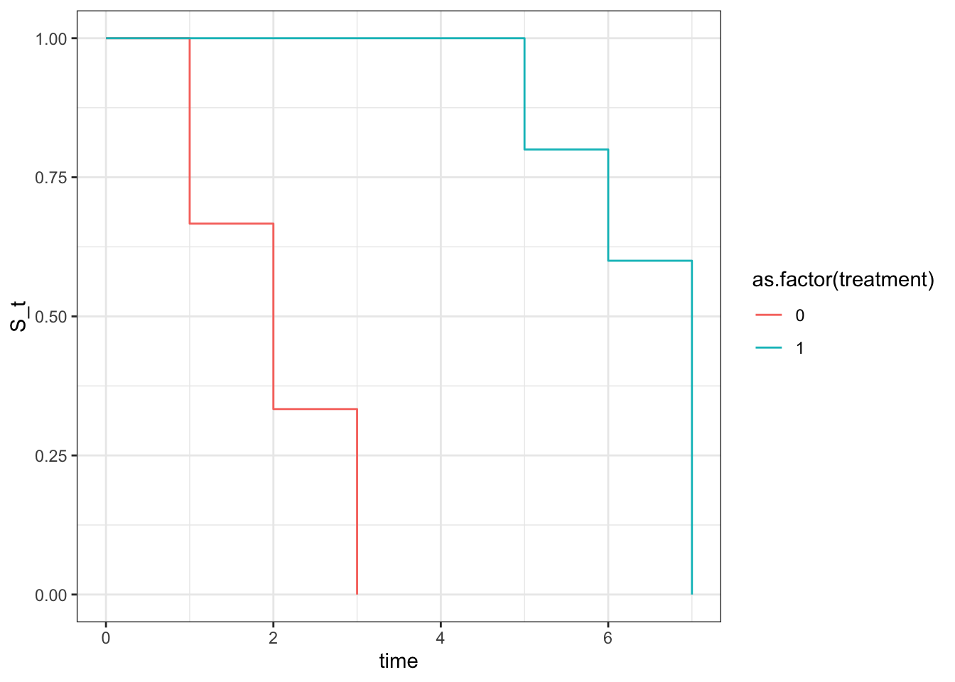
Wow, since we created this simpel dataset, knowing treatment extended the time event, whereas no treatment didn’t, we can nicely see that when creating 2 KM plots stratified by the treatment group and plot it all they look very different. Now let’s quickly look at log rank test with survival package and then calculate by hand and see if we can reproduce the same p value.
## log-rank test
(log_rank_test <- survival::survdiff(Surv(time, status) ~ treatment, data = simple_df))
## Call:
## survival::survdiff(formula = Surv(time, status) ~ treatment,
##     data = simple_df)
##
##             N Observed Expected (O-E)^2/E (O-E)^2/V
## treatment=0 6        5     1.97      4.68      9.02
## treatment=1 6        4     7.03      1.31      9.02
##
##  Chisq= 9  on 1 degrees of freedom, p= 0.003
Alright! It looks like a chi-square test and has a p val of 0.003. Let’s see if we can reproduce that. And it also looked like they use (O-E)^2/V as opposed to sum of (O-E)^2/E like the usual chi-square test to get the chisq statistic. Interesting.
V (variance) = n_0 * n_1 * d * (n - d) / (n^2 * (n - 1))
Click Here For Calculated Details
## log-rank test by hand
n0 <- 6
n1 <- 6

### time 1
simple_df |>
  filter(time == 1) |>
  group_by(treatment) |>
  summarize(n = n(),
            d = sum(status))
## # A tibble: 1 × 3
##   treatment     n     d
##       <dbl> <int> <dbl>
## 1         0     2     2
(t_1 <- tibble(n0=n0, n1=n1, d0=2, d1=0) |>
  mutate(n = n0 + n1) |>
  mutate(d = d0 + d1) |>
  mutate(V = n0 * n1 * d * (n - d) / (n^2 * (n - 1))) |>
  mutate(E0 = (n0 /n) * d) |>
  mutate(chi_i = (d0-E0)^2/V))
## # A tibble: 1 × 9
##      n0    n1    d0    d1     n     d     V    E0 chi_i
##   <dbl> <dbl> <dbl> <dbl> <dbl> <dbl> <dbl> <dbl> <dbl>
## 1     6     6     2     0    12     2 0.455     1   2.2
n0 <- n0 - 2
n1 <- n1 - 0

### time 2
simple_df |>
  filter(time == 2) |>
  group_by(treatment) |>
  summarize(n = n(),
            d = sum(status))
## # A tibble: 2 × 3
##   treatment     n     d
##       <dbl> <int> <dbl>
## 1         0     3     2
## 2         1     1     0
(t_2 <- tibble(n0=n0, n1=n1, d0=2, d1=0) |>
  mutate(n = n0 + n1) |>
  mutate(d = d0 + d1) |>
  mutate(V = n0 * n1 * d * (n - d) / (n^2 * (n - 1))) |>
  mutate(E0 = (n0 /n) * d) |>
  mutate(chi_i = (d0-E0)^2/V))
## # A tibble: 1 × 9
##      n0    n1    d0    d1     n     d     V    E0 chi_i
##   <dbl> <dbl> <dbl> <dbl> <dbl> <dbl> <dbl> <dbl> <dbl>
## 1     4     6     2     0    10     2 0.427   0.8  3.37
n0 <- n0 - 3
n1 <- n1 - 1

### time 3
simple_df |>
  filter(time == 3) |>
  group_by(treatment) |>
  summarize(n = n(),
            d = sum(status))
## # A tibble: 1 × 3
##   treatment     n     d
##       <dbl> <int> <dbl>
## 1         0     1     1
(t_3 <- tibble(n0=n0, n1=n1, d0=1, d1=0) |>
  mutate(n = n0 + n1) |>
  mutate(d = d0 + d1) |>
  mutate(V = n0 * n1 * d * (n - d) / (n^2 * (n - 1))) |>
  mutate(E0 = (n0 /n) * d) |>
  mutate(chi_i = (d0-E0)^2/V))
## # A tibble: 1 × 9
##      n0    n1    d0    d1     n     d     V    E0 chi_i
##   <dbl> <dbl> <dbl> <dbl> <dbl> <dbl> <dbl> <dbl> <dbl>
## 1     1     5     1     0     6     1 0.139 0.167     5
n0 <- n0 - 1
n1 <- n1 - 0

### time 5
simple_df |>
  filter(time == 5) |>
  group_by(treatment) |>
  summarize(n = n(),
            d = sum(status))
## # A tibble: 1 × 3
##   treatment     n     d
##       <dbl> <int> <dbl>
## 1         1     1     1
(t_5 <- tibble(n0=n0, n1=n1, d0=0, d1=1) |>
  mutate(n = n0 + n1) |>
  mutate(d = d0 + d1) |>
  mutate(V = n0 * n1 * d * (n - d) / (n^2 * (n - 1))) |>
  mutate(E0 = (n0 /n) * d) |>
  mutate(chi_i = (d0-E0)^2/V))
## # A tibble: 1 × 9
##      n0    n1    d0    d1     n     d     V    E0 chi_i
##   <dbl> <dbl> <dbl> <dbl> <dbl> <dbl> <dbl> <dbl> <dbl>
## 1     0     5     0     1     5     1     0     0   NaN
n1 <- n1 - 1

### time 6
simple_df |>
  filter(time == 6) |>
  group_by(treatment) |>
  summarize(n = n(),
            d = sum(status))
## # A tibble: 1 × 3
##   treatment     n     d
##       <dbl> <int> <dbl>
## 1         1     2     1
(t_6 <- tibble(n0=n0, n1=n1, d0=0, d1=1) |>
  mutate(n = n0 + n1) |>
  mutate(d = d0 + d1) |>
  mutate(V = n0 * n1 * d * (n - d) / (n^2 * (n - 1))) |>
  mutate(E0 = (n0 /n) * d) |>
  mutate(chi_i = (d0-E0)^2/V))
## # A tibble: 1 × 9
##      n0    n1    d0    d1     n     d     V    E0 chi_i
##   <dbl> <dbl> <dbl> <dbl> <dbl> <dbl> <dbl> <dbl> <dbl>
## 1     0     4     0     1     4     1     0     0   NaN
n1 <- n1 - 2

### time 7
simple_df |>
  filter(time == 7) |>
  group_by(treatment) |>
  summarize(n = n(),
            d = sum(status))
## # A tibble: 1 × 3
##   treatment     n     d
##       <dbl> <int> <dbl>
## 1         1     2     2
(t_7 <- tibble(n0=n0, n1=n1, d0=0, d1=2) |>
  mutate(n = n0 + n1) |>
  mutate(d = d0 + d1) |>
  mutate(V = n0 * n1 * d * (n - d) / (n^2 * (n - 1))) |>
  mutate(E0 = (n0 /n) * d) |>
  mutate(chi_i = (d0-E0)^2/V))
## # A tibble: 1 × 9
##      n0    n1    d0    d1     n     d     V    E0 chi_i
##   <dbl> <dbl> <dbl> <dbl> <dbl> <dbl> <dbl> <dbl> <dbl>
## 1     0     2     0     2     2     2     0     0   NaN
n1 <- n1 - 2
Alright, lots of back and forth sanity check but I think we did it! Now, let’s replace those NaN to 0, do some calculation and check our final chi square statistic
bind_rows(t_1, t_2, t_3, t_5, t_6, t_7) |>
  mutate(V = replace_na(V, 0),
         E0 = replace_na(E0, 0)) |>
  summarise(
    O0 = sum(d0),
    E0 = sum(E0),
    V  = sum(V)
  ) |>
  mutate(chi_sq = (O0 - E0)^2 / V)
## # A tibble: 1 × 4
##      O0    E0     V chi_sq
##   <dbl> <dbl> <dbl>  <dbl>
## 1     5  1.97  1.02   9.02
pchisq(q = 9.02, df = 1, lower.tail = F)
## [1] 0.002670414
🙌🙌🙌 We got it! If we round it up, it’s exactly 0.003 just like from survival.
Notice that we used E0, but you can use E1 and it would should return the same chi square statistic. Click below for details.
Click to expand
bind_rows(t_1, t_2, t_3, t_5, t_6, t_7) |>
  mutate(E1 = (n1 / n) * d) |>
  summarise(
    O1 = sum(d1),
    E1 = sum(E1),
    V = sum(V)
  ) |>
  mutate(chi_sq = (O1-E1)^2/V)
## # A tibble: 1 × 4
##      O1    E1     V chi_sq
##   <dbl> <dbl> <dbl>  <dbl>
## 1     4  7.03  1.02   9.02
Take note that KM estimator can only estimate survival function and you can only compare the survival curves with log-rank test, but you can’t add more variables to adjust for confounding. Which means, we assume that there isn’t any confounding factors between treatment groups.
If any adjustment that’s needed, that’s where Cox proportional hazard model comes in. Now if we were to add age and run cox model, we would get a different hazard ratio and p value, but the log-rank test would still be the same because log-rank test is only comparing the survival curves without adjusting for any covariates. Let’s see that in action. Click below to expand, you’re going to see an interesting warning, complete separation.
Click to Expand
simple_df <- tribble(
  ~time, ~status, ~treatment, ~age,
  5,1,1,30,
  2,1,0,80,
  6,0,1,35,
  1,1,0,85,
  2,0,1,32,
  2,0,0,30,
  7,1,1,25,
  3,1,0,90,
  7,1,1,98,
  2,1,0,98,
  1,1,0,89,
  6,1,1,20
) |>
  mutate(subject = row_number())

survival::coxph(Surv(time,status) ~ treatment+age, data = simple_df)
## Warning in coxph.fit(X, Y, istrat, offset, init, control, weights = weights, :
## Loglik converged before variable 1 ; coefficient may be infinite.
## Call:
## survival::coxph(formula = Surv(time, status) ~ treatment + age,
##     data = simple_df)
##
##                 coef  exp(coef)   se(coef)      z     p
## treatment -2.202e+01  2.729e-10  1.937e+04 -0.001 0.999
## age        2.275e-03  1.002e+00  1.192e-02  0.191 0.849
##
## Likelihood ratio test=10.61  on 2 df, p=0.004959
## n= 12, number of events= 9
Notice how our treatment has high p val, and high SE? Since our mock data has a clear separation between treatment and age, where all the treated patients are young and all the untreated patients are old, the model is having a hard time estimating the effect of treatment because it’s confounded by age. This is called complete separation, and it leads to infinite estimates for the coefficients, which is why we see those warnings. In real world data, we might not have such a clear separation, but we might still have some degree of separation that can lead to unstable estimates. That’s why it’s important to check for separation and consider using penalized regression methods if we encounter this issue.
Let’s simulate the data so that we can estimate a more accurate hazard ratio with cox model and see how it compares to the true hazard ratio that we set in the simulation.
Simulation
library(survival)
library(survminer)

# simulate data of HR 0.55 (95%CI 0.442-0.674)
set.seed(1)
n <- 350
base_event <- 25
base_rate <- 1/base_event
treatment_event <- base_event + 20
treatment_rate <- 1/treatment_event
hr <- treatment_rate/base_rate
coef <- log(hr)
confounder <- rbinom(n,1,0.5)
treatment <- rbinom(n, 1, plogis(0.5*confounder))
true_time <- rexp(n, rate = base_rate*exp(coef*treatment+0.5*confounder))
cens_time <- runif(n, min = 0, max = treatment_event)

df <- tibble(true_time, cens_time) |>
  mutate(time = pmin(true_time, cens_time),
         status = case_when(
           true_time <= cens_time ~ 1,
           TRUE ~ 0
         )) |>
  mutate(confounder = confounder) |>
  mutate(treatment = treatment |> as.factor())

head(df)
## # A tibble: 6 × 6
##   true_time cens_time  time status confounder treatment
##       <dbl>     <dbl> <dbl>  <dbl>      <int> <fct>
## 1     13.0      42.3  13.0       1          0 0
## 2      8.83      2.60  2.60      0          0 0
## 3      4.49     13.7   4.49      1          1 0
## 4     61.4      10.8  10.8       0          1 1
## 5     47.7      17.3  17.3       0          0 1
## 6     11.6      34.3  11.6       1          1 1
The above simulation, we set the true hazard ratio to be 0.55, which means that the treatment group has a 45% reduction in the hazard of the event compared to the control group. We then simulate the true time to event using an exponential distribution, and we also simulate a censoring time using a uniform distribution. The observed time is the minimum of the true time and the censoring time, and the status variable indicates whether the event was observed (1) or censored (0).
Simulating the above is helpful because we then know the true rate was derived from exponential function based on base rate multiplied by the hazard ratio, so we can then compare the estimated hazard ratio from the Cox model to the true hazard ratio we set in the simulation. The part that connects intuitively is how the exp(coef\*treatment+coef2\*confounder) is similar to the linear regression. If you noticed that we use base_rate*exp(...), it’s essentialy the same as exp(log(base_rate)+coef\*treatment+coef2\*confounder) which is the same as exp(intercept + coef\*treatment + coef2\*confounder), where the intercept is log(base_rate). So, in a way, the Cox model is modeling the log of the hazard function as a linear combination of the covariates, which is similar to how linear regression models the mean of the outcome as a linear combination of the covariates. The difference is that in Cox model, we are modeling the hazard function, which is the instantaneous rate of event occurrence at time t, whereas in linear regression, we are modeling the mean of the outcome variable.
Kaplan-Meier Estimator
(survdiff(Surv(time,status) ~ treatment, data = df))
## Call:
## survdiff(formula = Surv(time, status) ~ treatment, data = df)
##
##               N Observed Expected (O-E)^2/E (O-E)^2/V
## treatment=0 149       74     62.3      2.20      3.61
## treatment=1 201       87     98.7      1.39      3.61
##
##  Chisq= 3.6  on 1 degrees of freedom, p= 0.06
km_fit <- survfit(Surv(time, status) ~ treatment, data = df)
the log-rank test did show a difference between the two groups, though not statistically significant (likely not adequate n), which is expected since we set a true hazard ratio of 0.55 in the simulation. The Kaplan-Meier estimator will give us the estimated survival curves for each group, and we can visually compare them to see the difference in survival between the treatment and control groups.
Cox Proportional Hazard Model
cox_fit <- coxph(Surv(time, status) ~ treatment + confounder, data = df, x = T)
summary(cox_fit)
## Call:
## coxph(formula = Surv(time, status) ~ treatment + confounder,
##     data = df, x = T)
##
##   n= 350, number of events= 161
##
##               coef exp(coef) se(coef)      z Pr(>|z|)
## treatment1 -0.3730    0.6887   0.1603 -2.327  0.01999 *
## confounder  0.5024    1.6526   0.1605  3.130  0.00175 **
## ---
## Signif. codes:  0 '***' 0.001 '**' 0.01 '*' 0.05 '.' 0.1 ' ' 1
##
##            exp(coef) exp(-coef) lower .95 upper .95
## treatment1    0.6887     1.4521     0.503    0.9429
## confounder    1.6526     0.6051     1.207    2.2635
##
## Concordance= 0.582  (se = 0.024 )
## Likelihood ratio test= 13.34  on 2 df,   p=0.001
## Wald test            = 13.34  on 2 df,   p=0.001
## Score (logrank) test = 13.5  on 2 df,   p=0.001
# plot
ggsurvplot(
  fit = km_fit,
  data = df,
  # pval = TRUE,
  conf.int = TRUE,
  risk.table = TRUE,
  legend.labs = c("Control", "Treatment"),
  title    = "Kaplan-Meier Survival Curves"
)
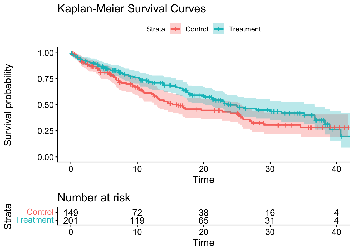
Notice how the estimated hazard ratio from the Cox model is close to the true hazard ratio of 0.55 that we set in the simulation, our HR is 0.595 (95% CI 0.44-0.81). The Kaplan-Meier plot showed us the survival curves for each group, and we can visually see the difference in survival between the treatment and control groups.
Note:
survdiffcalculates log-rank test,survfitestimates the survival function, andcoxphestimates the hazard ratio adjusting for covariates
There is an
interesting article by Hernán that cautioned the use of unadjusted HR and the use unadjusted survival curve (which we did, because it’s based off KM estimator). He also mentioned that first, a single average HR across the entire follow-up can be misleading because the true effect may vary over time. Let’s see if we can apply that to our current plot. Let’s use adjustedCurves and see if it looks different.
library(adjustedCurves)

adjust_curve <- adjustedsurv(
  data = df,
  ev_time = "time",
  event = "status",
  variable = "treatment",
  method = "direct",
  outcome_model = cox_fit,
  conf_int = T)

plot(adjust_curve, conf_int = T)
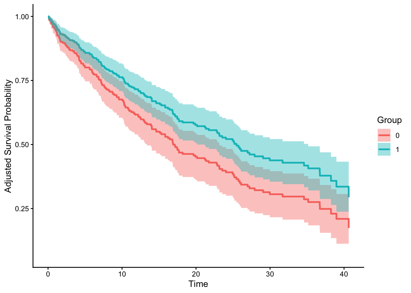
Interesting. They do look different! Though the paper didn’t directly use this package. He also proposed a solution to more accurately estimate time-varying HR using pooled logistic regression and spline on time as feature. Let’s try this next time! So much to learn! On
Emily Zabor’s blog, she did mention there is survival::cox.zph() function which allows us to check the assumption of proportional hazards.
Acknowledgement
Thanks to Emily Zabor’s tutorial and also personal advice on practical usage of survival analysis! Her blog contains so much more advanced topics and some functions and packages I’m planning to use in the future. It’s truly one of the more comprehensive and yet easy to understand tutorials I’ve seen on survival analysis. Thanks Emily!
Also thanks to John Blishak for pointing out some of the typos and url error. I’ve made those changes as well. Thanks, John! I was telling him that LLM wouldn’t have made those rookie error lol.
Opportunities For Improvement
- learn competing risk analysis with fine-gray model
- learn to customize ggsurvplot
- use
gtsummary::tbl_regression(exp = TRUE)to further beautify aHR - test out Hernán’s proposed solution to calculate HR
- let’s test out other dataset such as BMT from SemiCompRisks, Melanoma from MASS,
Lessons learnt
- calculating by hand is helpful because I just realized we can’t just calculate at_risk with one row at a time because of the time occurs at the same time, it would be calculated at the same time, that’s why we used for loop for clarity
survdiffcalculates log-rank test,survfitestimates the survival function, andcoxphestimates the hazard ratio adjusting for covariates- censor is usually a good thing, but it could also mean lost to follow up.
If you like this article:
- please feel free to send me a comment or visit my other blogs
- please feel free to follow me on BlueSky, twitter, GitHub or Mastodon
- if you would like collaborate please feel free to contact me
- Posted on:
- May 2, 2026
- Length:
- 19 minute read, 3992 words