V_s__l_ng M_ss_ng D_t_ W_th D_G & S_m_l_t__n
By Ken Koon Wong in r R missing mar mnar mcar dag
June 22, 2024
MCAR, MAR, MNAR, all so confusing.
But with DAG, oh so amusing!
Many technical words, I don’t understand,
but with simulation, I am a fan!
Join me in exploring missing mechanisms,
learn I will with great optimism.
Visualizing Missing Data With DAG & Simulation

Just for kicks, what is the missing mechanism of the title? Scroll all the way down for answer!
Motivations
The motivation behind this topic stems from the attempt to understand the missing mechanisms of Missing Completely At Random (MCAR), Missing At Random (MAR), and Missing Not At Random (MNAR). I had a hard time understanding its terminology and also definition, until I stumbled upon Understanding missing data mechanisms using causal DAGs mechanism by Cameron Patrick. Very informative and also has a lot of references to guide my journey of simulating these mechanisms in order for me to grasp the surface of the meaning of missingness. It was a bumpy road, and I must say, I don’t think I completely understand it, but I think I’m getting closer. Disclaimer, this is a note for myself with R code to generate the missing mechanisms for all 3 properties and also the underlying mathematical notation. If you find any mistakes in my understanding, please feel free to comment below and guide me to the right path.
Objectives
- Motivations
- Generate Data
- MCAR
- MAR
- MNAR
- Variety of Missingness DAGs/notation/representation
- Opportunity for Improvement
- References
- Lessons Learnt
Generate Data
library(tidyverse)
library(broom)

set.seed(1)
n <- 100
z <- rnorm(n)
x <- 0.2*z + rnorm(n)
y <- 0.3*z + 0.5*x + rnorm(n)

model <- lm(y~x+z)

summary(model)
##
## Call:
## lm(formula = y ~ x + z)
##
## Residuals:
##      Min       1Q   Median       3Q      Max
## -2.94359 -0.43645  0.00202  0.63692  2.63941
##
## Coefficients:
##             Estimate Std. Error t value Pr(>|t|)
## (Intercept)  0.02535    0.10519   0.241  0.81005
## x            0.44653    0.10948   4.079 9.29e-05 ***
## z            0.33180    0.11877   2.794  0.00628 **
## ---
## Signif. codes:  0 '***' 0.001 '**' 0.01 '*' 0.05 '.' 0.1 ' ' 1
##
## Residual standard error: 1.043 on 97 degrees of freedom
## Multiple R-squared:  0.2339,	Adjusted R-squared:  0.2181
## F-statistic: 14.81 on 2 and 97 DF,  p-value: 2.442e-06
A very simple continuous data for x (exposure), y (outcome), and z (common cause). We aren’t going to pay too much attention to z on the DAG, hence it’s omitted, so that we can focus on the missingness mechanism.
Take note that the true x coefficient is 0.4465332 and the std.error is 0.1094785.
Now let’s write a function so that we can visualize the missing values of the different missingness mechanisms we’re about to encounter.
Write a function to Visualize
compare_plot <- function(z=z,x=x,y=y,ym=ym,mechanism) {
  df <- tibble(y,x,z,ym)

 plot <- ggplot() +
  geom_point(df, mapping=aes(x=x,y=y), color = "red", alpha = 0.5) +
  geom_smooth(df, mapping=aes(x=x,y=y), method = "lm", color = "black") +
  geom_point(df, mapping=aes(x=x,y=ym), color = "blue", alpha = 0.5) +
  geom_smooth(df, mapping=aes(x=x,y=ym), method = "lm", color = "red") +
   ggtitle(label = mechanism, subtitle = paste0("y observed (blue point), y missing (red point), true x coef (black line), \nx coef with y missing (red line)")) +
   theme_bw()

 return(plot)
}
MCAR

X: Exposure.
Y: Complete outcome, sometimes this is also the sum of Y_mis (missing Y) and Y_obs(observed Y).
Yobs: Outcome that is observed.
M: Missingness mechanism of Y, sometimes can be represented as My
\begin{gather} P(M=0|Y_{obs},Y_{mis},\psi) = P(M=0|\psi) \end{gather}
Over here, we assign M = 0 as missing, where M = 1 is not missing.
Take note that this on certain textbooks are reversed. Let \(\psi\) contain the parameters of the missing data model. With MCAR missing mechanism, we can ignore \(Y_{obs}\) and \(Y_{mis}\), hence it’s the missingness is random, not caused by variables in the DAG. Example in real life could be data missing from a portable meter due to out of battery.
Alright, let’s similate this in R and visualize it! Take note that when we estimate X coefficient, we will be using complete case analysis (aka listwise deletion, pairwise deletion, available case analysis, deletion methods, complete record analysis). We will not attempt to impute at this point.
# mcar
my <- rbinom(n, 1, 0.7) |> as.logical()

ym <- c()

for (i in 1:n) {
  ym[i] <- ifelse(my[i]==T,y[i],NA)
}

summary(lm(ym ~ x + z))
##
## Call:
## lm(formula = ym ~ x + z)
##
## Residuals:
##      Min       1Q   Median       3Q      Max
## -2.88370 -0.62185 -0.02348  0.67784  2.80147
##
## Coefficients:
##             Estimate Std. Error t value Pr(>|t|)
## (Intercept) -0.02645    0.12961  -0.204  0.83894
## x            0.43957    0.14479   3.036  0.00341 **
## z            0.45181    0.14763   3.060  0.00318 **
## ---
## Signif. codes:  0 '***' 0.001 '**' 0.01 '*' 0.05 '.' 0.1 ' ' 1
##
## Residual standard error: 1.08 on 67 degrees of freedom
##   (30 observations deleted due to missingness)
## Multiple R-squared:  0.2798,	Adjusted R-squared:  0.2583
## F-statistic: 13.01 on 2 and 67 DF,  p-value: 1.678e-05
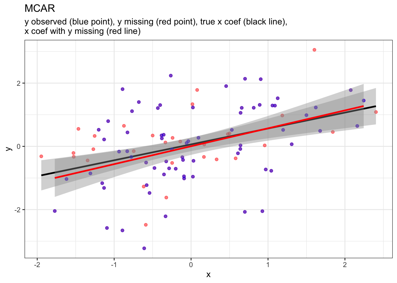
compare_plot(z,x,y,ym,"MCAR")

What’s going on up there? Let’s break it down. We assigned my with random variable of a binomial distribution with a probability of 70%. So that means, about 70% of the time we will see 1, which we had said before that M = 0 will be our missingness mechanism, that means 30% will be missing, randomly. Then, we turn these ones and zeros to logical data. Next, we create an empty vector ym to slot in data when My == T, else assign NA. Then we estimate our model with observed data.
Our X coefficient is quite close to the real one. 🙌 though with 30% of data missing, you can see that the confidence interval is much wider than the original data. This is also known as
loss of precision (increasing the uncertainty of the estimations).
MAR

As you can see on the DAG above, M is affected by X. That means the missingness mechanism is not completely at random. Something else caused it. The mathematical notation would be:
\begin{gather} P(M=0|Y_{obs},Y_{mis},\psi) = P(M=0|Y_{obs},\psi) \end{gather}
The missingness mechanism is the probability of missingness depends on the observed information of any design factor, which also means for MAR, we can ignore Y_mis, and hence our mechanism is \(P(M=0|Y_{obs},\psi)\). Now let’s simulate and visualize!
# MAR
my <- rbinom(n,1,plogis(2-2*x)) |> as.logical()

for (i in 1:n) {
  ym[i] <- ifelse(my[i]==T,y[i],NA)
}

summary(lm(ym~x+z))
##
## Call:
## lm(formula = ym ~ x + z)
##
## Residuals:
##     Min      1Q  Median      3Q     Max
## -2.8750 -0.3840  0.0631  0.6970  1.8169
##
## Coefficients:
##             Estimate Std. Error t value Pr(>|t|)
## (Intercept)  -0.1665     0.1279  -1.302 0.196810
## x             0.2158     0.1596   1.352 0.180365
## z             0.5004     0.1288   3.886 0.000218 ***
## ---
## Signif. codes:  0 '***' 0.001 '**' 0.01 '*' 0.05 '.' 0.1 ' ' 1
##
## Residual standard error: 0.9926 on 75 degrees of freedom
##   (22 observations deleted due to missingness)
## Multiple R-squared:  0.2172,	Adjusted R-squared:  0.1964
## F-statistic: 10.41 on 2 and 75 DF,  p-value: 0.0001026
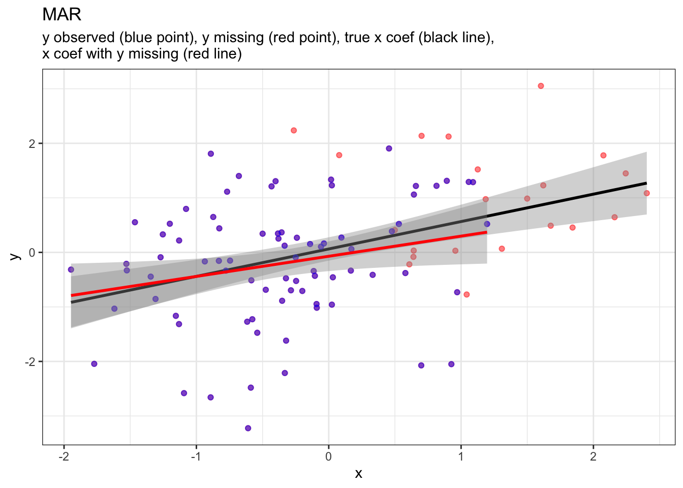
compare_plot(z,x,y,ym,"MAR")

Let’s explain. We assigned my now with the influence of x and then turn it into boolean. Same procedure, if my is TRUE, then slot in data, if not, make it NA. Our estimation now is, same as MCAR, imprecise, with a wider confidence interval, and also the X coefficient is different from the true estimate. Same thing with the intercept as well. Usually, it is advised that we impute these numbers so that we don’t throw out data.
MNAR / NMAR

\begin{gather} P(M=0|Y_{obs},Y_{mis},\psi) = P(M=0|Y_{obs},Y_{mis},\psi) \end{gather}
Now, this is a very interesting one! I never understood this until I can visualize this on a DAG. Anytime when the variable itself (that is missing) affects the missingness mechanism, it’s MNAR! Another name for MNAR is also Not Missing At Random (NMAR). In real life example would be missing lactate results in patients. For example, lactate is usually not ordered when not indicated, which also usually means the the lactate value is most likely normal or low. Hence, low/normal value of lactate will likely to go missing. Imputation in this setting may produce a biased result.
my <- rbinom(n,1,plogis(-2*x+2*y)) |> as.logical()

for (i in 1:n) {
  ym[i] <- ifelse(my[i]==T,y[i],NA)
}

summary(lm(ym~x+z))
##
## Call:
## lm(formula = ym ~ x + z)
##
## Residuals:
##      Min       1Q   Median       3Q      Max
## -1.74498 -0.59748  0.02568  0.60912  2.15993
##
## Coefficients:
##             Estimate Std. Error t value Pr(>|t|)
## (Intercept)   0.5183     0.1362   3.805 0.000364 ***
## x             0.6595     0.1502   4.391 5.29e-05 ***
## z             0.2861     0.1286   2.224 0.030329 *
## ---
## Signif. codes:  0 '***' 0.001 '**' 0.01 '*' 0.05 '.' 0.1 ' ' 1
##
## Residual standard error: 0.8888 on 54 degrees of freedom
##   (43 observations deleted due to missingness)
## Multiple R-squared:  0.3624,	Adjusted R-squared:  0.3388
## F-statistic: 15.34 on 2 and 54 DF,  p-value: 5.287e-06
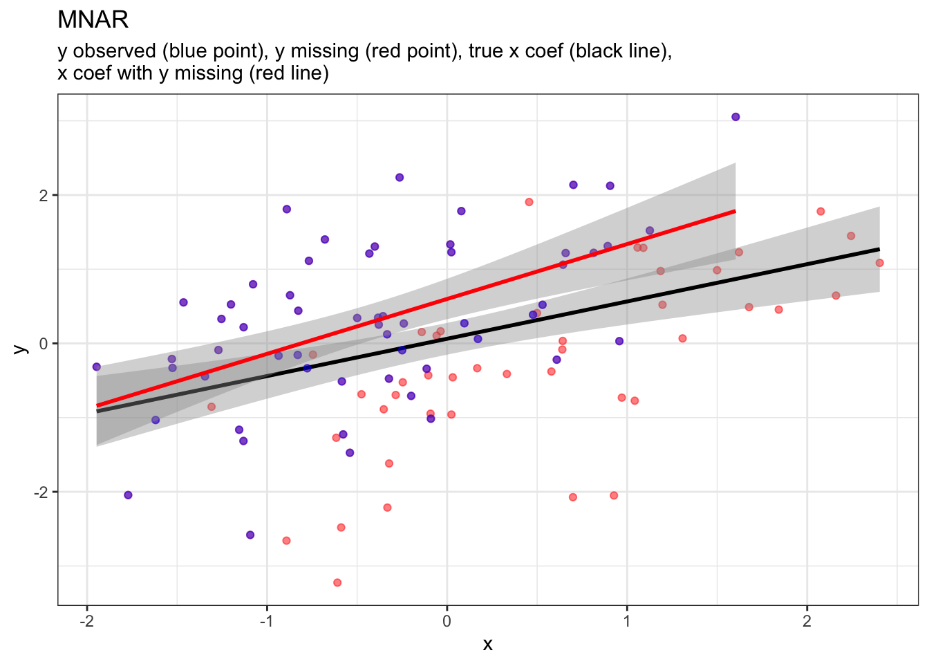
compare_plot(z,x,y,ym,"MNAR")

Now our estimate is REALLY off! Complete case analysis here is not appropriate at all.
Different variety of Missing Data DAGs/notation/representation
DAG
-
Enders, Craig K.. Applied Missing Data Analysis (Methodology in the Social Sciences Series) (p. 6). Guilford Publications.
 This is the DAG that we have adopted on this article.
 -
Statistical Rethinking by Richard McElreath
 Here, Richard uses a concept of dog (missingness mechanism) eating homework as an example. Hence,
 Dis the missingness mechanism. Otherwise looks quite similar to our DAG. -
[Canonical Causal Diagrams to Guide the Treatment of Missing Data in Epidemiologic] Studies( https://doi.org/10.1093/aje/kwy173)

Where represents unmeasured variables which affect the missingness mechanism that are not affected by any of the variables in the study. Missingness mechanisms of the variable were prefixed byM, for exampleMyindicated missingness mechanism ofYvariable,MxofX,Mz1ofZ2.
Representation
Through out the blog, we assign M = 0 as missing, where M = 1 is not missing. But different textbooks will have this reversed. Hence, missingness notation/representation and also DAGs are not universally consistent.
Opportunity for improvement
- Next time, we will explore a bit more on the solutions to each missingness mechanisms, what is recoverability, ignorabiity? Which imputation technique to use, what kinds are there?
- If MNAR is a non-outcome or exposure variable, does it matter much?
- use
ggdagto draw DAGs next time instead of copy and pasting fromdagitty
References
- Understanding missing data mechanisms using causal DAGs
- van Buuren, Stef. Flexible Imputation of Missing Data, Second Edition (Chapman & Hall/CRC Interdisciplinary Statistics) (p. 36). CRC Press.
- Enders, Craig K.. Applied Missing Data Analysis (Methodology in the Social Sciences Series) (p. 6). Guilford Publications.
- [Canonical Causal Diagrams to Guide the Treatment of Missing Data in Epidemiologic] Studies( https://doi.org/10.1093/aje/kwy173)
Lessons Learnt
- Missingness notation/representation/DAGs are not universally consistent. We have presented a few versions above.
- We learnt what MCAR, MAR, and MNAR mean through DAG and simulation
- [Canonical Causal Diagrams to Guide the Treatment of Missing Data in Epidemiologic] Studies( https://doi.org/10.1093/aje/kwy173) is a great resource! Full of information
Answer: The missingness mechanism of the title is… MNAR. Only vowels were missing, meaning vowels caused the title to be missing vowels.
If you like this article:
- please feel free to send me a comment or visit my other blogs
- please feel free to follow me on twitter, GitHub or Mastodon
- if you would like collaborate please feel free to contact me
- Posted on:
- June 22, 2024
- Length:
- 9 minute read, 1865 words