Exploring Interaction Effects and S-Learners
By Ken Koon Wong in r R interaction meta learner s learner boost tree lightgbm
September 4, 2023
Interaction adventures through simulations and gradient boosting trees using the S-learner approach. I hadn’t realized that lightGBM and XGBoost could reveal interaction terms without explicit specification. Quite intriguing!
 picture resembles
 interaction 🤣
Objectives:
- What is interaction?
- Simulate interaction
- Visualize interaction
- True Model ✅
- Wrong Model ❌
- What is S Learner?
- What is CATE?
- Boost Tree Model
- Limitation
- Acknowledgement
- Lessons Learnt
What is interaction?
In statistics, interaction refers to the phenomenon where the effect of one variable on an outcome is influenced by the presence or change in another variable. It indicates that the relationship between variables is not simply additive, but rather depends on the interaction between their values. Understanding interactions is crucial for capturing complex relationships and building accurate predictive models that consider the combined influence of variables, providing deeper insights into data analysis across various fields.
Still don’t understand? No worries, you’re not alone. I’ve been there too! However, I found that simulating and visualizing interactions really helped solidify my understanding of their significance. Missing out on understanding interactions is like skipping a few chapters in the story – it’s an essential part of grasping the whole picture.
Simulate interaction
library(tidymodels)
library(tidyverse)
library(bonsai)
library(kableExtra)
library(ggpubr)

set.seed(1)
n <- 1000
x1 <- rnorm(n)
x2 <- rnorm(n)
x3 <- rnorm(n)
y1 <- 0.2*x1 + rnorm(n)
y2 <- 1 + 0.6*x2 + rnorm(n)
y3 <- 2 + -0.2*x3 + rnorm(n)

# combining all y_i to 1 vector
y <- c(y1,y2,y3)

# categorize x1, x2, and x3
df <- tibble(y=y,x=c(x1,x2,x3),x_i=c(rep("x1",n),rep("x2",n),rep("x3",n)))

kable(df |> head(5))
| y | x | x_i |
|---|---|---|
| 0.6138242 | -0.6264538 | x1 |
| 0.4233374 | 0.1836433 | x1 |
| 1.1292714 | -0.8356286 | x1 |
| -0.4845022 | 1.5952808 | x1 |
| -1.5367241 | 0.3295078 | x1 |
But hold on, Ken, that’s not interaction, right? Doesn’t interaction involve terms like y = x + w + x*w? Well, yes, you’re right about that equation, but the explanation above offers a more intuitive grasp of what interaction entails. It’s like taking the nominal categories x1, x2, x3, treating them as on-off switches, and then consolidating all three equations into one primary equation. This approach helps in calculating the interrelationships between them. Trust me. Also this was a great
resource in understanding the interaction formula too.
This is essentially our formula:
\(Y_i = B_0 + B_1X_{1i} + B_2X_{2i} + B_3X_{3i} + B_4X_{1i}X_{2i} + B_5X_{1i}X_{3i} + e_i\).
Wow, there are too many \(B\)’s. I can see why it is hard to follow. We’ll carry this formula with us and unpack it later on.
Visualize interaction
df |>
  ggplot(aes(x=x,y=y,color=as.factor(x_i))) +
  geom_point(alpha = 0.5) +
  geom_smooth(method = "lm") +
  theme_minimal()
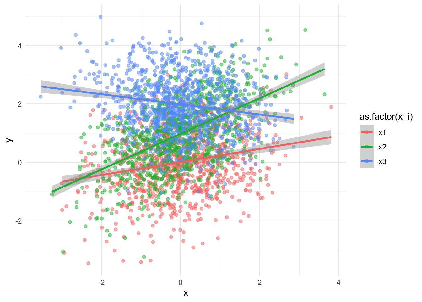
Wow, look at those slopes of x1, x2, x3. We can all agree that they all have different intercepts and slopes. That my friend, is interaction.
True Model ✅
model_true <- lm(y~x*x_i,df)
summary(model_true)
##
## Call:
## lm(formula = y ~ x * x_i, data = df)
##
## Residuals:
##     Min      1Q  Median      3Q     Max
## -3.6430 -0.6684 -0.0105  0.6703  3.0552
##
## Coefficients:
##             Estimate Std. Error t value Pr(>|t|)
## (Intercept)  0.01700    0.03172   0.536    0.592
## x            0.22356    0.03066   7.291 3.91e-13 ***
## x_ix2        0.96309    0.04486  21.471  < 2e-16 ***
## x_ix3        1.97089    0.04486  43.938  < 2e-16 ***
## x:x_ix2      0.38554    0.04325   8.913  < 2e-16 ***
## x:x_ix3     -0.39672    0.04344  -9.133  < 2e-16 ***
## ---
## Signif. codes:  0 '***' 0.001 '**' 0.01 '*' 0.05 '.' 0.1 ' ' 1
##
## Residual standard error: 1.003 on 2994 degrees of freedom
## Multiple R-squared:  0.4465,	Adjusted R-squared:  0.4455
## F-statistic:   483 on 5 and 2994 DF,  p-value: < 2.2e-16
Intercepts of x1, x2, and x3
 Notice that the first intercept is the first equation of
 y1 = x1 + noise and the intercept should be zero, or at least close to zero. The second intercept is x2’s. Notice that in the equation that simulates the data has a 1 as intercept? Where does this recide in the true model? Yes you’re right, on x_ix2 ! It’s not 1 but it’s close to 1. And the third intercept for x3 is on x_ix3.
What if intercept for x1 is not zero? Read on below.
Slopes of x1, x2, and x3
 What about the slopes? the slope for
 x1 is on x, x2 is on x:x_ix2, x3 is on x:x_ix3. The interaction is the slope! How cool! Wait, you may say, they don’t add up! x2 coefficient should be 0.6 but why is x:x_ix2 about 0.22 less? Wait a minute, does 0.22 of coefficient look familiar to you? It’s x1’s coefficient (or in this case listed as x).
Wowowow, hold the phone, so the slopes for x2 is the sum of x1 coefficient and x:x_ix2 the interaction term !?! YES, precisely! And the same would be for x3 too? Let’s do the math, 0.224 + (-0.397) = -0.173 which is very close to -0.2 which is the true x3 coefficient! And you can even see the negative slope from the visualization too (represented by blue color). Superb! 🙌
So, if the intercept x1 is not zero, it’s the same thing as the slope coefficients, you just simply add them up! How neat to be able to combine all 3 equations (of the same measurements of course, meaning y and x are measuring the same things) into 1 equation!
Wrong Model ❌
model_wrong <- lm(y~x + x_i,df)
summary(model_wrong)
##
## Call:
## lm(formula = y ~ x + x_i, data = df)
##
## Residuals:
##     Min      1Q  Median      3Q     Max
## -3.9952 -0.7085 -0.0088  0.7068  3.4459
##
## Coefficients:
##             Estimate Std. Error t value Pr(>|t|)
## (Intercept)  0.01698    0.03339   0.509    0.611
## x            0.22206    0.01863  11.922   <2e-16 ***
## x_ix2        0.95681    0.04721  20.265   <2e-16 ***
## x_ix3        1.96486    0.04722  41.614   <2e-16 ***
## ---
## Signif. codes:  0 '***' 0.001 '**' 0.01 '*' 0.05 '.' 0.1 ' ' 1
##
## Residual standard error: 1.056 on 2996 degrees of freedom
## Multiple R-squared:  0.3862,	Adjusted R-squared:  0.3856
## F-statistic: 628.4 on 3 and 2996 DF,  p-value: < 2.2e-16
Notice that if we only naively model y and x relationship without taking account to the interaction terms, we’re not seeing the whole picture. We’ll be missing out the actual slopes and falsely thinking that x_ix3 is the slope, when it is supposed to be negative.
If we were to visualize it would be something like this
df |>
  ggplot(aes(x=x,y=y,color=x_i)) +
  geom_point() +
  geom_abline(intercept = model_wrong$coefficients[[1]], slope = model_wrong$coefficients[["x"]], color = "red") +
  geom_abline(intercept = model_wrong$coefficients[[1]], slope = model_wrong$coefficients[["x_ix2"]], color = "green") +
  geom_abline(intercept = model_wrong$coefficients[[1]], slope = model_wrong$coefficients[["x_ix3"]], color = "blue") +
  theme_minimal()
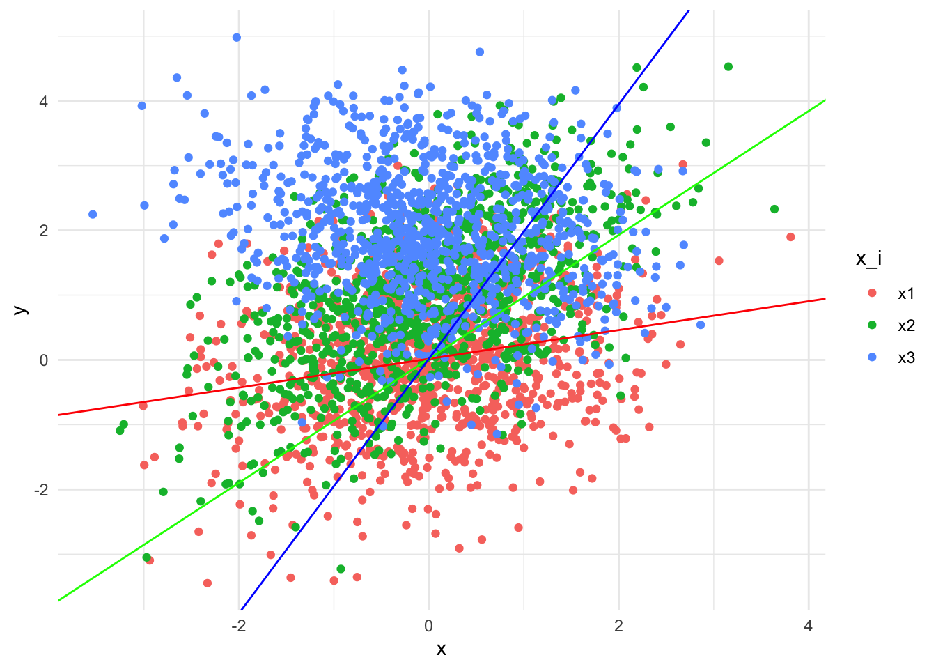
Doesn’t look right, does it?
What is S Learner?
S-learner is one of the early Machine Learning Meta-learners that can be used for estimating the conditional average treatment effect (CATE) in causal inference. The simplest in my opinion, which is great, makes us understand the other Meta-learners better, such as T, X, R, DL, after understanding how to construct this one first. We basically take treatment variable just like any other covariate, train the model with a machine learning model of your choice, and then use that to estimate CATE, all in ONE model!
Response function:
\(\mu(x,z) := \mathbb{E}(Y^{obs}|X=x,Z=z)\)
Estimate CATE by:
\(\hat{t}(x) = \mu(X=1,Z=z) - \mu(X=0, Z=z)\)
$\mu$: Model of choice.
Y: Outcome.
X: binary treatment variable.
Z: other covariates. Though, we don’t have any in our current simulation.
$\hat{t}$: CATE
For excellent explaination on S-learner please check this link by José Luis Cañadas Reche and this link on Statistical Odds & Ends.
What is CATE?
Conditional Average Treatment Effect (CATE) is a foundational concept in causal inference, focusing on the difference in expected outcomes between individuals who receive a treatment and those who do not, while considering their unique characteristics or covariates. Representing the average impact of treatment while accounting for individual differences, CATE helps answer how treatments influence outcomes in a given context. It’s calculated as the difference between the expected outcomes under treatment and no treatment conditions for individuals with specific covariate values, providing crucial insights into causal relationships and guiding decision-making across various domains.
Boost Tree Model
I’m a great supporter of tidymodels. In this context, we’ll utilize this framework to apply boosting tree methods and determine whether they can reveal interaction terms without requiring explicit specification. For S-learner, we basically will use a model, train with all data, then use the model to calculate CATE.
Light GBM
#split
# split <- initial_split(df, prop = 0.8)
# train <- training(split)
# test <- testing(split)

#preprocess
rec <- recipe(y ~ ., data = df) |>
  step_dummy(all_nominal())

rec |> prep() |> juice() |> head(5) |> kable()
| x | y | x_i_x2 | x_i_x3 |
|---|---|---|---|
| -0.6264538 | 0.6138242 | 0 | 0 |
| 0.1836433 | 0.4233374 | 0 | 0 |
| -0.8356286 | 1.1292714 | 0 | 0 |
| 1.5952808 | -0.4845022 | 0 | 0 |
| 0.3295078 | -1.5367241 | 0 | 0 |
#cv
cv <- vfold_cv(data = df, v = 5, repeats = 5)

#engine
gbm <- boost_tree() |>
  set_engine("lightgbm") |>
  set_mode("regression")


#workflow
gbm_wf <- workflow() |>
  add_recipe(rec) |>
  add_model(gbm)

#assess
gbm_assess <- gbm_wf %>%
  fit_resamples(
    resamples = cv,
    metrics = metric_set(rmse, rsq, ccc),
    control = control_resamples(save_pred = TRUE, verbose = TRUE)
  )

gbm_assess |>
  collect_metrics() |> kable()
| .metric | .estimator | mean | n | std_err | .config |
|---|---|---|---|---|---|
| ccc | standard | 0.5971348 | 25 | 0.0028353 | Preprocessor1_Model1 |
| rmse | standard | 1.0401944 | 25 | 0.0054528 | Preprocessor1_Model1 |
| rsq | standard | 0.4072577 | 25 | 0.0033576 | Preprocessor1_Model1 |
#fit
gbm_fit <- gbm_wf |>
  fit(df)
Alright, let’s use default hyperparameters without tuning lightbgm and see how things go. Observe that during our preprocessing, we did not specify interaction terms such as y ~ x*x_i.
Let’s look at our True Model CATE of x2 comparing to x1 when x is 3 ✅
predict(model_true, newdata=tibble(x=3,x_i="x2")) - predict(model_true, newdata=tibble(x=3,x_i="x1"))
##        1
## 2.119704
Let’s look at our Wrong Model CATE of x2 comparing to x1 when x is 3 ❌
predict(model_wrong, newdata=tibble(x=3,x_i="x2")) - predict(model_wrong, newdata=tibble(x=3,x_i="x1"))
##         1
## 0.9568113
Let’s look at LightGBM CATE of x2 comparing to x1 when x is 3. 🌸
predict(gbm_fit, new_data=tibble(x=3,x_i="x2")) - predict(gbm_fit, new_data=tibble(x=3,x_i="x1"))
##      .pred
## 1 1.952928
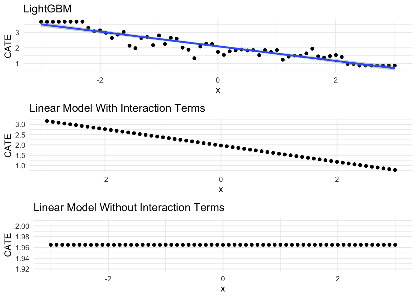
Wow, LightGBM is quite close to the tru model. Let’s sequence a vector of x and assess all 3 models.
# write a function
assess <- function(model,x,x_i,x_base="x1") {
  if (class(model)!="workflow") {
    diff <- predict(model, newdata=tibble(x=!!x,x_i=!!x_i)) - predict(model, newdata=tibble(x=!!x,x_i=x_base))
  } else {
  diff <- (predict(model, new_data=tibble(x=!!x,x_i=!!x_i)) - predict(model, new_data=tibble(x=!!x,x_i=x_base))) |> pull() }
  return(tibble(x=!!x,diff=diff))
}

# sequence of x's
x <- seq(-3,3,0.1)

# type of x_i of interest
x_i <- "x2"

gbm_g<- assess(model=gbm_fit,x=x,x_i=x_i) |>
  ggplot(aes(x=x,y=diff)) +
  geom_point() +
  # geom_smooth(method="lm") +
  theme_minimal() +
  ggtitle("LightGBM") +
  ylab("CATE")

true_g <- assess(model=model_true,x=x,x_i=x_i) |>
  ggplot(aes(x=x,y=diff)) +
  geom_point()  +
  theme_minimal() +
  ggtitle("Linear Model With Interaction Terms") +
  ylab("CATE")

wrong_g <- assess(model=model_wrong,x=x,x_i=x_i) |>
  ggplot(aes(x=x,y=diff)) +
  geom_point()  +
  theme_minimal() +
  ggtitle("Linear Model Without Interaction Terms") +
  ylab("CATE")

ggarrange(gbm_g,true_g,wrong_g, ncol = 1)
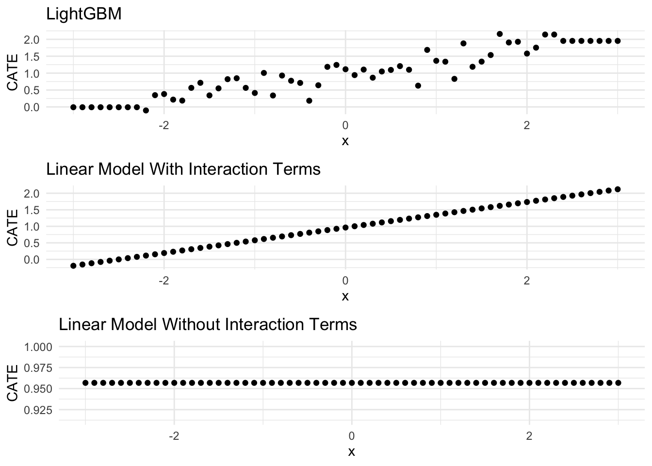
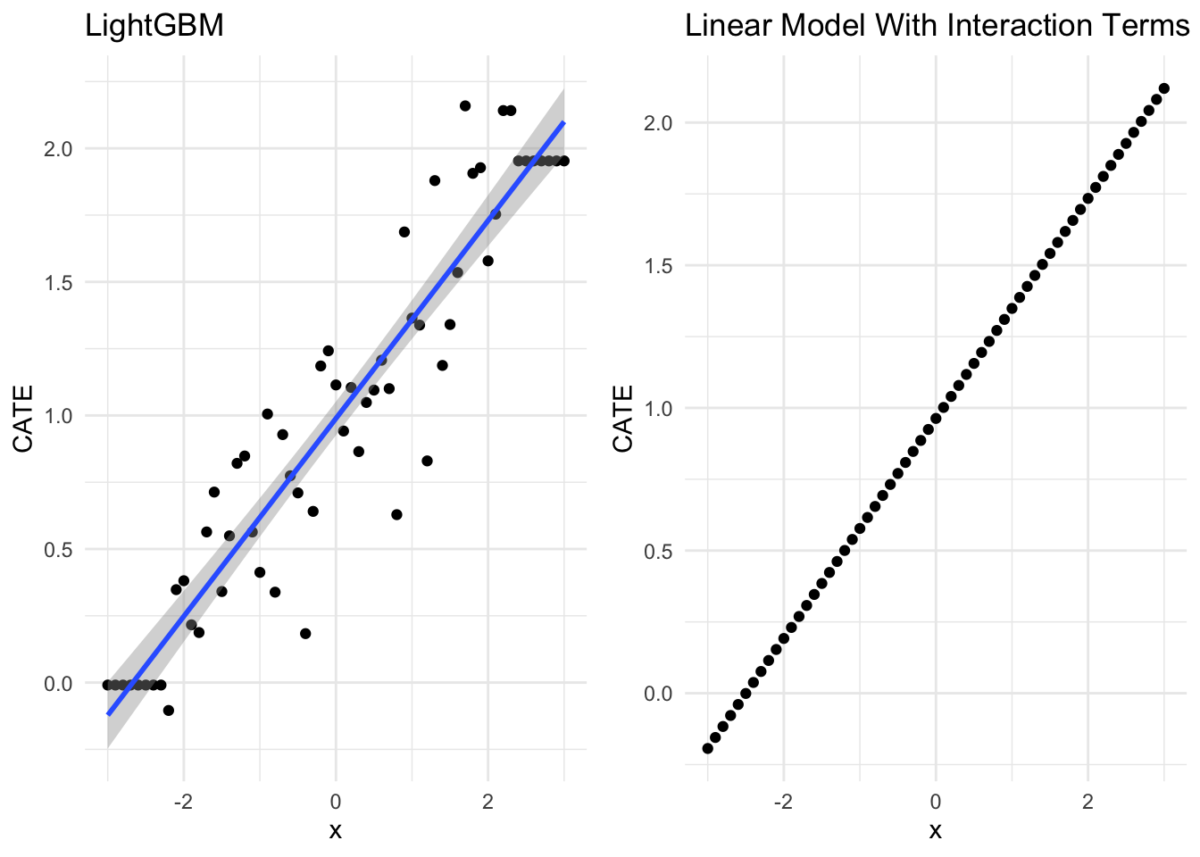
Very interesting indeed! LightGBM seems to be able to get very similar CATE compared to True model! The sequence of prediction by LightGBM also looks quite familiar, doesn’t it? If we were to use its prediction regressing on x, it looks like the slope might be very similar to the true model. Let’s give a a try
LightGBM’s CATE regressing on x
gbm_pred <- assess(gbm_fit, x = x, x_i = "x2")
summary(lm(diff~x,gbm_pred))
##
## Call:
## lm(formula = diff ~ x, data = gbm_pred)
##
## Residuals:
##      Min       1Q   Median       3Q      Max
## -0.65741 -0.10984 -0.01303  0.13675  0.54059
##
## Coefficients:
##             Estimate Std. Error t value Pr(>|t|)
## (Intercept)  0.98884    0.03152   31.38   <2e-16 ***
## x            0.37032    0.01790   20.69   <2e-16 ***
## ---
## Signif. codes:  0 '***' 0.001 '**' 0.01 '*' 0.05 '.' 0.1 ' ' 1
##
## Residual standard error: 0.2462 on 59 degrees of freedom
## Multiple R-squared:  0.8788,	Adjusted R-squared:  0.8768
## F-statistic:   428 on 1 and 59 DF,  p-value: < 2.2e-16
True model’s CATE regressing on x
model_true_pred <- assess(model_true, x, "x2")
summary(lm(diff~x,model_true_pred))
##
## Call:
## lm(formula = diff ~ x, data = model_true_pred)
##
## Residuals:
##        Min         1Q     Median         3Q        Max
## -2.883e-15 -2.088e-17  3.261e-17  7.979e-17  2.103e-15
##
## Coefficients:
##              Estimate Std. Error   t value Pr(>|t|)
## (Intercept) 9.631e-01  6.155e-17 1.565e+16   <2e-16 ***
## x           3.855e-01  3.496e-17 1.103e+16   <2e-16 ***
## ---
## Signif. codes:  0 '***' 0.001 '**' 0.01 '*' 0.05 '.' 0.1 ' ' 1
##
## Residual standard error: 4.808e-16 on 59 degrees of freedom
## Multiple R-squared:      1,	Adjusted R-squared:      1
## F-statistic: 1.216e+32 on 1 and 59 DF,  p-value: < 2.2e-16
very very similar indeed! Let’s visualize them side by side
gbm_g<- assess(model=gbm_fit,x=x,x_i=x_i) |>
  ggplot(aes(x=x,y=diff)) +
  geom_point() +
  geom_smooth(method="lm") +
  theme_minimal() +
  ggtitle("LightGBM") +
  ylab("CATE")

ggarrange(gbm_g,true_g)
What if we look at x3?
# sequence of x's
x <- seq(-3,3,0.1)

# type of x_i of interest
x_i <- "x3"

gbm_g<- assess(model=gbm_fit,x=x,x_i=x_i) |>
  ggplot(aes(x=x,y=diff)) +
  geom_point() +
  geom_smooth(method="lm") +
  theme_minimal() +
  ggtitle("LightGBM") +
  ylab("CATE")

true_g <- assess(model=model_true,x=x,x_i=x_i) |>
  ggplot(aes(x=x,y=diff)) +
  geom_point()  +
  theme_minimal() +
  ggtitle("Linear Model With Interaction Terms") +
  ylab("CATE")

wrong_g <- assess(model=model_wrong,x=x,x_i=x_i) |>
  ggplot(aes(x=x,y=diff)) +
  geom_point()  +
  theme_minimal() +
  ggtitle("Linear Model Without Interaction Terms") +
  ylab("CATE")

ggarrange(gbm_g,true_g,wrong_g, ncol = 1)
XGBoost
gbb <- boost_tree() |>
  set_engine("xgboost") |>
  set_mode("regression")

#workflow
gbb_wf <- workflow() |>
  add_recipe(rec) |>
  add_model(gbb)

#assess
gbb_assess <- gbb_wf %>%
  fit_resamples(
    resamples = cv,
    metrics = metric_set(rmse, rsq, ccc),
    control = control_resamples(save_pred = TRUE, verbose = TRUE)
  )

gbb_assess |>
  collect_metrics() |> kable()
| .metric | .estimator | mean | n | std_err | .config |
|---|---|---|---|---|---|
| ccc | standard | 0.5968061 | 25 | 0.0031061 | Preprocessor1_Model1 |
| rmse | standard | 1.0318791 | 25 | 0.0057834 | Preprocessor1_Model1 |
| rsq | standard | 0.4144199 | 25 | 0.0038228 | Preprocessor1_Model1 |
gbb_fit <- gbb_wf |>
  fit(df)

# sequence of x's
x <- seq(-3,3,0.1)

# type of x_i of interest
x_i <- "x2"

gbb_g<- assess(model=gbb_fit,x=x,x_i=x_i) |>
  ggplot(aes(x=x,y=diff)) +
  geom_point() +
  geom_smooth(method="lm") +
  theme_minimal() +
  ggtitle("LightGBM") +
  ylab("CATE")

true_g <- assess(model=model_true,x=x,x_i=x_i) |>
  ggplot(aes(x=x,y=diff)) +
  geom_point()  +
  theme_minimal() +
  ggtitle("Linear Model With Interaction Terms") +
  ylab("CATE")

ggarrange(gbb_g,true_g)
x_i <- "x3"

gbb_g<- assess(model=gbb_fit,x=x,x_i=x_i) |>
  ggplot(aes(x=x,y=diff)) +
  geom_point() +
  geom_smooth(method="lm") +
  theme_minimal() +
  ggtitle("LightGBM") +
  ylab("CATE")

true_g <- assess(model=model_true,x=x,x_i=x_i) |>
  ggplot(aes(x=x,y=diff)) +
  geom_point()  +
  theme_minimal() +
  ggtitle("Linear Model With Interaction Terms") +
  ylab("CATE")

ggarrange(gbb_g,true_g)
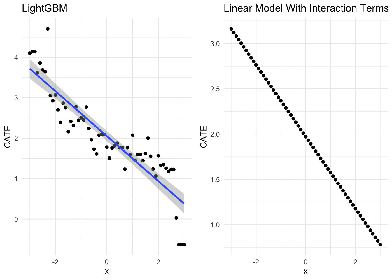
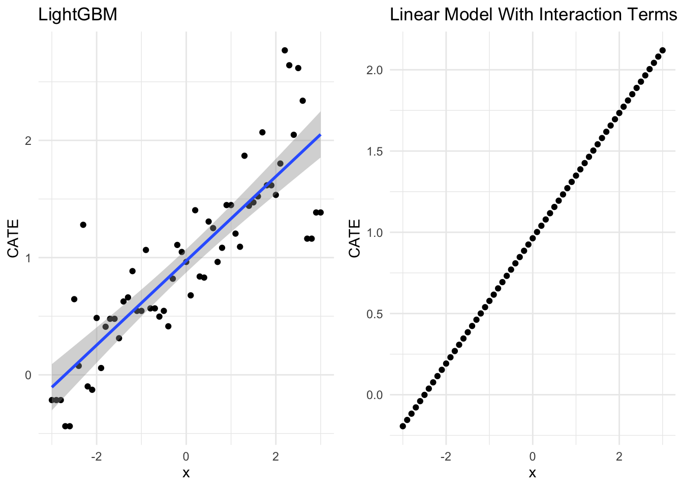
Not too shabby either!

Limitation
- We haven’t truly added confounders such as
zto the mix, we’ll hae to see how that pans out with interaction. I sense another blog coming up! - We may not be actually be using the S-learner method in the right setting. It’s usually to assess a binary treatment and its outcome. Here we’re focused more on interaction terms and how boost tree can tease that out.
- If you see any mistakes or any comments, please feel free to reach out!
Acknowledgement
- Thanks to José Luis Cañadas Reche’s inspiring S-learner blog, please check this link. I wasn’t planning on doing interaction and S-learner at the same time, but this gave me an opportunity.
- Barr, Dale J. (2021). Learning statistical models through simulation in R: An interactive textbook really helped me to understand interaction
- Last but not least, Aleksander Molak’s book is awesome and learnt about Meta-learners.
Lessons Learnt
geom_ablineto draw custom line based on intercept + slopes\mathbb{E}symbol for Expected in LaTeX- Gradient boosting models such as
lightGBMcan tease out interaction, quite a handy tool! - Learnt what interaction is and how to interpret its summary
- Learnt S-learner
If you like this article:
- please feel free to send me a comment or visit my other blogs
- please feel free to follow me on twitter, GitHub or Mastodon
- if you would like collaborate please feel free to contact me
- Posted on:
- September 4, 2023
- Length:
- 12 minute read, 2526 words
- Categories:
- r R interaction meta learner s learner boost tree lightgbm