An Educational Stroll With Stan - Part 2
By Ken Koon Wong in r R stan cmdstanr bayesian beginner
September 28, 2023
I learned a great deal throughout this journey. In the second part, I gained knowledge about implementing logistic regression in Stan. I also learned the significance of data type declarations for obtaining accurate estimates, how to use posterior to predict new data, and what generated quantities in Stan is for. Moreover, having a friend who is well-versed in Bayesian statistics proves invaluable when delving into the Bayesian realm! Very fun indeed!

We’ve looked at linear regression previously, now let’s take a look at logistic regression.
Objectives
- Load Library & Simulate Simple Data
- What Does A Simple Logistic Regression Look Like In Stan?
- Visualize It!
- How To Predict Future Data ?
- Acknowledgement/Fun Fact
- Lessons Learnt
Load Library & Simulate Simple Data
library(tidyverse)
library(cmdstanr)
library(bayesplot)
library(kableExtra)

set.seed(1)
n <- 1000
w <- rnorm(n)
x <- rbinom(n,1,plogis(-1+2*w))
y <- rbinom(n,1,plogis(-1+2*x + 3*w))
collider <- -0.5*x + -0.6*y + rnorm(n)
df <- list(N=n,x=x,y=y,w=w, collider=collider) #cmdstanr uses list
df2 <- tibble(x,y,collider,w) #this is for simple logistic regression check

Same DAG as
before but the difference is both x and y are binary via binomial distribution.
Look At GLM summary
model <- glm(y ~ x + w, df2, family = "binomial")
summary(model)
##
## Call:
## glm(formula = y ~ x + w, family = "binomial", data = df2)
##
## Deviance Residuals:
##      Min        1Q    Median        3Q       Max
## -2.93224  -0.42660  -0.06937   0.29296   2.79793
##
## Coefficients:
##             Estimate Std. Error z value Pr(>|z|)
## (Intercept)  -1.0352     0.1240  -8.348   <2e-16 ***
## x             2.1876     0.2503   8.739   <2e-16 ***
## w             2.9067     0.2230  13.035   <2e-16 ***
## ---
## Signif. codes:  0 '***' 0.001 '**' 0.01 '*' 0.05 '.' 0.1 ' ' 1
##
## (Dispersion parameter for binomial family taken to be 1)
##
##     Null deviance: 1375.9  on 999  degrees of freedom
## Residual deviance:  569.2  on 997  degrees of freedom
## AIC: 575.2
##
## Number of Fisher Scoring iterations: 6
Nice! x and w coefficients and y intercept are close to our simulated model! x coefficient is 2.1875657 (true: 2), w coefficient is 2.9066911 (true:3).
What About Collider?
model2 <- lm(collider ~ x + y, df2)
summary(model2)
##
## Call:
## lm(formula = collider ~ x + y, data = df2)
##
## Residuals:
##     Min      1Q  Median      3Q     Max
## -3.5744 -0.6454 -0.0252  0.7058  2.8273
##
## Coefficients:
##              Estimate Std. Error t value Pr(>|t|)
## (Intercept)  0.007275   0.044300   0.164     0.87
## x           -0.461719   0.090672  -5.092 4.23e-07 ***
## y           -0.610752   0.086105  -7.093 2.48e-12 ***
## ---
## Signif. codes:  0 '***' 0.001 '**' 0.01 '*' 0.05 '.' 0.1 ' ' 1
##
## Residual standard error: 1.032 on 997 degrees of freedom
## Multiple R-squared:  0.1753,	Adjusted R-squared:  0.1736
## F-statistic: 105.9 on 2 and 997 DF,  p-value: < 2.2e-16
Not too shabby. x coefficient is -0.4617194 (true: -0.5), y coefficient is -0.6107524 (true: -0.6). Perfect! But how do we do this on Stan?
Let’s break down what exactly we want to estimate.
\begin{gather} y\sim\text{bernoulli}(p) \\ \text{logit}(p) = a_y+b_{yx}.x+b_{yw}.w \\ \\ collider\sim\text{normal}(\mu_{collider},\sigma_{collider}) \\ \mu_{collider}=a_{collider}+b_{collider\_x}.x+b_{collider\_y}.y \end{gather}
we’re basically interested in \(a_y\), \(b_{yx}\), \(b_{yw}\), \(a_{collider}\), \(b_{collider\_x}\), \(b_{collider\_y}\). To see if they reflect the parameters set in our simulation.
Logistic Regression via Stan
data {
  int N;
  array[N] int x;
  array[N] int y;
  array[N] real w; #note that this is not int but real
  array[N] real collider; #same here
}

parameters {
  // parameters for y (bernoulli)
  real alpha_y;
  real beta_yx;
  real beta_yw;

  // parameters for collider (normal)
  real alpha_collider;
  real beta_collider_x;
  real beta_collider_y;
  real sigma_collider;
}

model {
  // prior
  // default for real will be uniform distribution

  // likelihood
     y ~ bernoulli_logit(alpha_y + beta_yx * to_vector(x) + beta_yw * to_vector(w));
     collider ~ normal(alpha_collider + beta_collider_x * to_vector(x) + beta_collider_y * to_vector(y), sigma_collider);

}
Save the above under log_sim.stan.Note that we didn’t have to use inverse_logit, bernoulli_logit nicely turn that equation into inverse logit for us.
Did you also notice that data declaration has array[N] (data type) (variable) instead of variable[N]. This is the new way of declaring the structure in Stan.
Run The Model in R and Analyze
mod <- cmdstan_model("log_sim.stan")

fit <- mod$sample(data = df,
                  chains = 4,
                  iter_sampling = 2000,
                  iter_warmup = 1000,
                  seed = 123,
                  parallel_chains = 4
                  )

fit$summary()

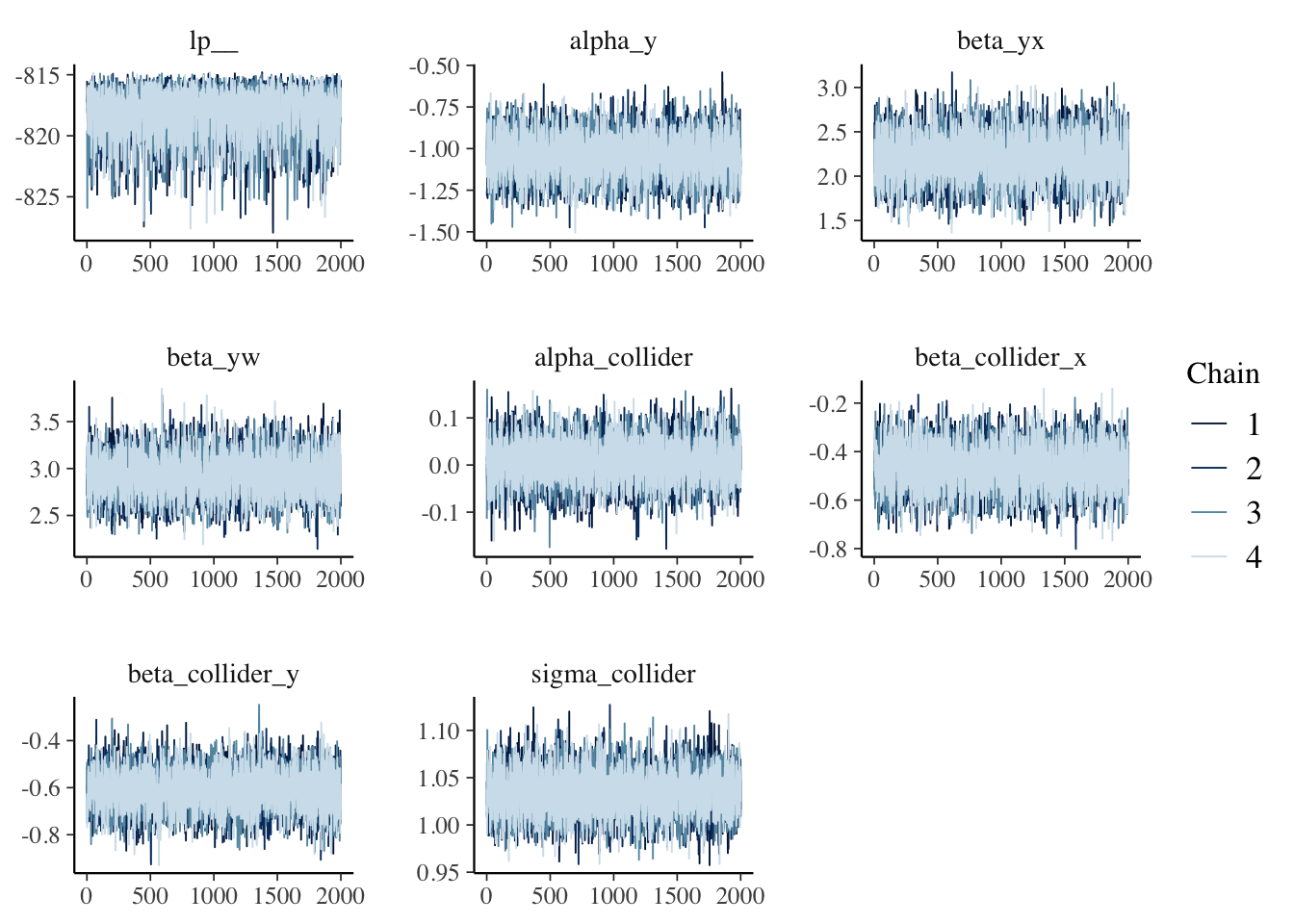
Not too shabby either! Stan model accurately estimated the alpha_y, beta_yx, beta_yw, alpha_collider, beta_collider_x, beta_collider_y parameters. Rhat is 1, less than 1.05. ess_bulk & ess_tail are >100. Model diagnostic looks good!
Visualize The Beautiful Convergence
mcmc_trace(fit$draws())

How To Predict Future Data ?
You know how in R or python, you can save the model and then type something like predict and the probability will miraculously appear? Well, to my knowledge, you can’t in Stan or cmdstanr. I heard you can with rstanarm, rethinking, brms etc. But let’s roll with it and see how we can do this.
Instructions:
- Extract your coefficient of interest from posterior
- Write another Stan model with generated quantities
- Feed New Data onto the Stan model and extract the expected value.
Recall this was our formula:
\begin{gather} y\sim\text{bernoulli}(p) \\ \text{logit}(p) = a_y+b_{yx}.x+b_{yw}.w \end{gather}
We want to extract alpha_y, beta_yx, and beta_yw.
Let’s Estimate y
#Extract parameters and then mean it
alpha_y <- fit$draws(variables = "alpha_y") |> mean()
beta_yx <- fit$draws(variables = "beta_yx") |> mean()
beta_yw <- fit$draws(variables = "beta_yw") |> mean()

#new data
set.seed(2)
n <- 100
x <- rbinom(n,1,0.5) #randomly assign a 1 for x
w <- rnorm(n) #randomly generate a continuous data for w
df_new <- list(N=n,x=x,w=w,alpha_y=alpha_y,beta_yx=beta_yx,beta_yw=beta_yw)
New Stan model
data {
  int<lower=0> N;
  array[N] int x;
  array[N] real w;
  real alpha_y;
  real beta_yx;
  real beta_yw;
}

// parameters {
//   array[N] real y_pred;
// }

generated quantities {
  array[N] real<lower=0,upper=1> y_pred;

  for (i in 1:N) {
    y_pred[i] = inv_logit(alpha_y + beta_yx * x[i] + beta_yw * w[i]);
}
}
Save the above to log_sim_pred.stan.
Note that this time, instead of declaring the model equation, we provided equation on generated quantities which essentially calculates the y_pred according to our formula.
Load Prediction Stan Model
mod <- cmdstan_model("log_sim_pred.stan")

fit2 <- mod$sample(data = df_new,
                  iter_sampling = 1,
                  chains =1,
                  fixed_param = T)
Notice that we provided df_new as data, changed iter_sampling to 1, if not we’ll just get a bunch of same numbers. Give it a try yourself! same goes with chains, additional chains of same values provide no additional value. Lastly, we have to specify fixed_param.
Merge Predicted y and True y
# create df with y_pred
df_pred <- as.data.frame(fit2$draws(variables = "y_pred")) |>
  pivot_longer(cols = everything(), names_to = "y_pred1", values_to = "y_pred") |>
  select(y_pred)

# create df w y_actual
df_actual <- tibble(x=x,w=w,y_actual=plogis(-1+2*x + 3*w)) |>
  select(y_actual)

# merge the 2 dfs and check the diff
df_combined <- df_pred |>
  add_column(df_actual) |>
  mutate(diff = y_actual - y_pred)

# load the first 5 rows
df_combined |>
  head(5) |>
  kable()
| y_pred | y_actual | diff |
|---|---|---|
| 0.029370 | 0.0288923 | -0.0004777 |
| 0.999270 | 0.9992532 | -0.0000168 |
| 0.382207 | 0.3347584 | -0.0474486 |
| 0.936812 | 0.9441253 | 0.0073133 |
| 0.129852 | 0.1050137 | -0.0248383 |
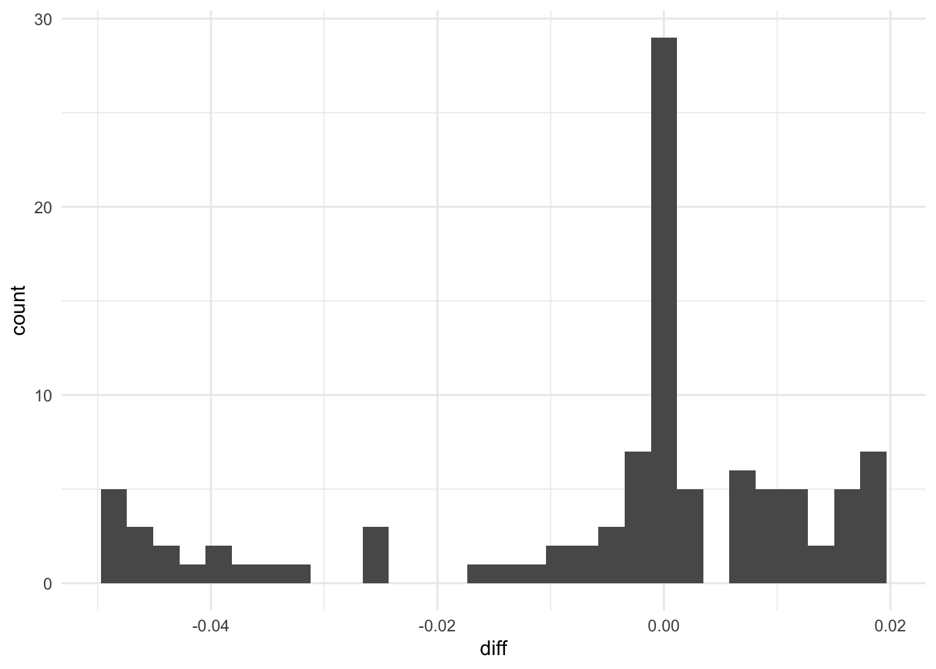
Not too shabby! Differences are quite small for the first 5. Let’s histogram it and see.
df_combined |>
  ggplot(aes(x=diff)) +
  geom_histogram() +
  theme_minimal()
Visualize Predicted and Actual y
df_combined |>
  ggplot(aes(x=y_actual,y=y_pred)) +
  geom_point() +
  geom_smooth(formula = "y ~ x") +
  theme_minimal()
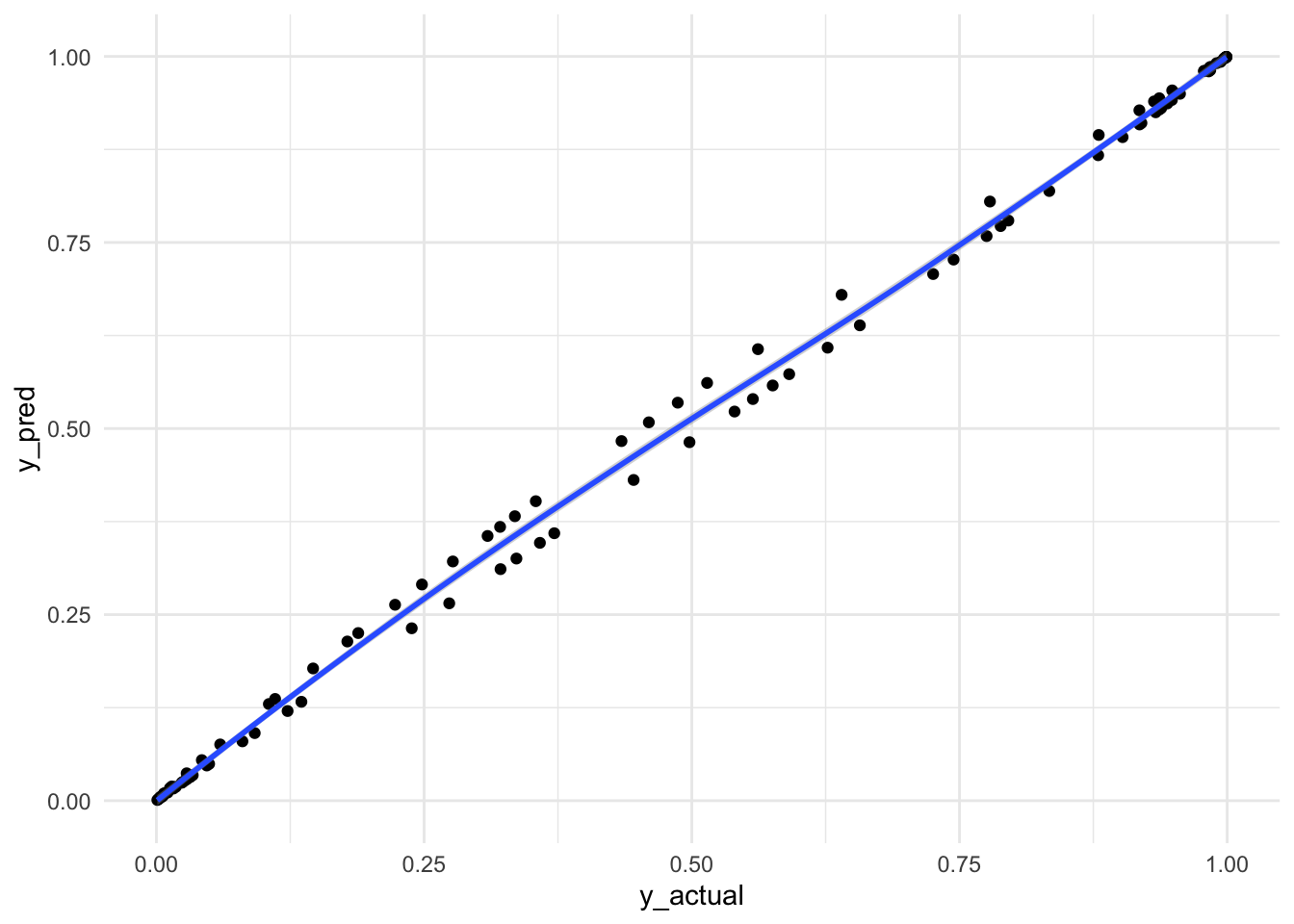
Almost a straight line through. Awesomeness! Not really sure why between 0.25 and 0.75 there were up down pattern. If you know, please let me know!
Acknowledgement/Fun Fact:
I truly want to thank Alec Wong for helping me with a problem I encountered. Initially my estimates were off, especially the collider parameters. Spent a few days and was not able to find out the cause. When you run into problem, stop and work on something else, or ask a friend! I did both! Alec Wong wrote a JAGS model and was able to extract accurate estimates. He sent me the script, we fed the script into chatGPT to spit out a Stan model and then realized that my data declaration had a mistake! Well, 2 mistakes! I put both w and collider as int instead of real. Here are the estiamtes when both w and collider were declared as int.

Notice how the collider parameters are off !?!?! The 95% credible intervals don’t even contain the true value.
Again, THANK YOU ALEC !!!
Things To Improve On:
- Will explore further using informed prior in the future
- Will explore simulated data of sens/spec of a diagnostic test and then apply prior to obtain posterior
- Will explore how Stan behaves with NULL data variable.
Lessons learnt:
- Learnt how to do logistic regression using cmdstanr
- Declaration of data type is important in Stan to get accurate estimates
- Stan has changed y[n] to array[n] y
- Learnt from Alec that rnorm(n, mu, sigma) == mu + rnorm(n, 0, sigma)
- Stan Manual is a good reference to go to
If you like this article:
- please feel free to send me a comment or visit my other blogs
- please feel free to follow me on twitter, GitHub or Mastodon
- if you would like collaborate please feel free to contact me
- Posted on:
- September 28, 2023
- Length:
- 7 minute read, 1485 words