An Educational Stroll With Stan - Part 1
By Ken Koon Wong in r R stan cmdstanr bayesian beginner
September 19, 2023
There is a lot to learn about Bayesian statistics, but it’s fun, exciting, and flexible! I thoroughly enjoyed the beginning of this journey. There will be learning curves, but there are so many great people and resources out there to help us get closer to understanding the Bayesian way.

Objectives
- What Is Stan?
- Load Library & Simulate Simple Data
- What Does A Simple Linear Regression Look Like?
- Visualize It!
- Things to Improve On/Learn
- Acknowledgement
- Lessons Learnt
What is Stan?
Stan is a probabilistic programming language used for statistical modeling and data analysis. It is particularly useful for Bayesian statistics. Stan provides a high-level interface for constructing complex statistical models and allows for robust, efficient sampling from the posterior distribution using Markov Chain Monte Carlo (MCMC) methods like the Hamiltonian Monte Carlo (HMC) algorithm or its adaptive variant, the No-U-Turn Sampler (NUTS).
Stan is highly expressive, meaning that users can specify a wide range of models without having to worry about the details of how the sampling is performed. Once the model is specified, Stan’s inference engine can estimate the parameters of the model given the data.
Stan is used in a variety of fields such as economics, epidemiology, social science research, machine learning, and many others. It offers interfaces to multiple programming languages including R (RStan), Python (PyStan), and Julia, allowing users to integrate Stan into a variety of data analysis workflows.
What Are Blocks in Stan?
Program structure is organized into specific blocks, each serving a distinct role in statistical modeling. The key blocks include data, which declares the known data; parameters, which declares the model’s variables to be estimated; transformed data and transformed parameters, which allow for the definition and transformation of data and parameters, respectively; model, where the statistical model and log probability function are defined; and generated quantities, where additional variables or quantities of interest can be calculated post-sampling. These blocks work in tandem to offer a complete specification for Bayesian inference.
All blocks are optional but must appear in a predefined order if they do occur. Variables declared in earlier blocks are available for use in later blocks, following specific scoping rules. For instance, a variable declared in the transformed data block can be used in the model block but not vice versa. Additionally, user-defined functions can be introduced in a functions block and can be used across different blocks. This structured approach makes Stan a flexible and powerful tool for a broad range of statistical modeling tasks.
Directly from Stan Documentations
functions {
  // ... function declarations and definitions ...
}
data {
  // ... declarations ...
}
transformed data {
   // ... declarations ... statements ...
}
parameters {
   // ... declarations ...
}
transformed parameters {
   // ... declarations ... statements ...
}
model {
   // ... declarations ... statements ...
}
generated quantities {
   // ... declarations ... statements ...
}
In our simple example, we will use only data, parameters, and model.
Load Library & Simulate Data
# Installation
# install.packages("cmdstanr", repos = c("https://mc-stan.org/r-packages/", getOption("repos")))

# Load libraries
library(cmdstanr)
library(tidyverse)
library(bayesplot)

set.seed(1)
n <- 1000
w <- rnorm(n)
x <- 0.5*w + rnorm(n)
y <- 0.2*x + 0.3*w + rnorm(n)
collider <- -0.5*x + -0.6*y + rnorm(n)
df <- list(N=n,x=x,y=y,w=w, collider=collider) # notice that we're using list instead of tibble/dataframe

In this example, we will be using cmdstanr.
With the above DAG, let’s break down what exactly we want to estimate.
\begin{gather} y \sim \text{normal}(\mu_y, \sigma_y) \\ \mu_y = a_y + b_{yx}.x + b_{yw}.w \\ collider \sim \text{normal}(\mu_{collider}, \sigma_{collider}) \\ \mu_{collider} = a_{collider} + b_{collider\_x}.x + b_{collider\_w}.w \end{gather}
The parameters we want to estimate would be \(a_y\), \(b_{yx}\), \(b_{yw}\), \(a_{collider}\), \(b_{collider\_x}\), \(b_{collider\_w}\)
Create A Stan Model:
data {
  // Declare data variable explicitly in stan model
  int<lower=0> N;
  vector[N] x;
  vector[N] y;
  vector[N] w;
  vector[N] collider;
}

parameters {
  // Declare parameters we want to estimate
  real a_y;
  real b_yx;
  real b_yw;
  real a_collider;
  real b_collider_x;
  real b_collider_y;
  real<lower=0> sigma_y;
  real<lower=0> sigma_collider;
  }
model {

  // Write out the model
  y ~ normal(a_y + b_yx * x + b_yw * w, sigma_y);
  collider ~ normal(a_collider + b_collider_x * x + b_collider_y * y, sigma_collider);
}
Run The Model in R and Analyze
# Create model object
mod <- cmdstan_model("lr.stan")

# Fit model
fit <- mod$sample(data = df,
                  iter_sampling = 2000,
                  iter_warmup = 1000, # how many iter to discard up front
                  chains = 4,
                  seed = 123,
                  save_warmup =  T, # I saved this because I'm curious about the output
                  parallel_chains = 4)
After you run the above code, the mcmc process would look something like this:

Look At Summary 📊
fit$summary()
 Wow, the estimate coefficients are very close to the true coefficients!
 b_yx is 0.216 (true: 0.2), b_yw is 0.322 (true: 0.3), b_collider_x is -0.502 (true: -0.5), b_collider_y is -0.591 (true: -0.6). Pretty good! ✅
But, what on earth are Rhat, ess_bulk, and ess_tail !?!?!?! 😱
What is Rhat? 🧢
The R-hat value is a measure used to check if the simulation chains in a Bayesian analysis have “converged” or come together well. In simple terms, it helps you understand if your model has settled into a stable solution. If the R-hat value is larger than 1, that suggests that the chains have not mixed well, meaning the model might not be reliable. Ideally, you should aim for an R-hat value less than 1.05 to trust the model’s results.
R-hat, specifically, compares the variance within each chain to the variance between different chains. If the chains have converged to the target distribution, the within-chain and between-chain variances should be approximately the same, leading to an R-hat value close to 1.
In simple terms, R-hat checks if different simulation runs (chains) are producing similar results. If they are, this gives you more confidence that your model has converged to a good estimate.
What Does Convergence Mean? 🤔
In simple terms, “convergence” means that the model has settled down and is now giving consistent results. It means that it has found a stable solution and you can trust the answers it’s giving you.
Imagine you’re trying to find the average height of people in a city by asking random people on the street. At first, after asking just a few people, your average might be way off—maybe you happened to ask some unusually tall or short people. But as you ask more and more people, your average will settle down to a more accurate and consistent number. When that happens, you’ve “converged” on an answer.
In MCMC, it’s a bit like that. The model starts with a guess and then improves it little by little. “Convergence” means the model has stopped guessing and is now consistently giving the same answer.
This is a great youtube link on the topic “Have I converged?”
What are ESS_bulk and ESS_tail?
The ess_bulk function helps you understand how well you’ve sampled the “middle” or “main part” of a distribution. In other words, it tells you how reliable your estimates are for the average and middle values of the data you’re studying. It does this by calculating a number called the Bulk Effective Sample Size (bulk-ESS).
The ess_tail function focuses on the “edges” or “tails” of the distribution. It calculates a number known as the Tail Effective Sample Size (tail-ESS). This number helps you understand how reliable your estimates are for the more extreme values and the spread of the data.
For both of these calculations, it’s generally a good idea to have a result of at least 100 per Markov Chain to feel confident that your estimates are reliable.
So, in simpler terms, ess_bulk tells you how good your sampling is for the main part of your data, and ess_tail tells you how good your sampling is for the extreme parts. And you want both of these numbers to be at least 100 to make sure your results can be trusted.
Visualize The MCMC Chains and Parameters
mcmc <- fit$draws(inc_warmup = T)

mcmc_df <- as.data.frame(mcmc) |>
  mutate(iter = row_number()) |>
  pivot_longer(cols = c(`1.lp__`:`4.sigma_collider`), names_to = "variable", values_to = "value") |>
  separate(col = "variable", into = c("chain","variable"), sep = "\\.")

mcmc_df |>
  ggplot(aes(x=iter,y=value,color=chain)) +
  geom_line(alpha=0.5) +
  facet_wrap(.~variable, scales = "free") +
  theme_minimal()

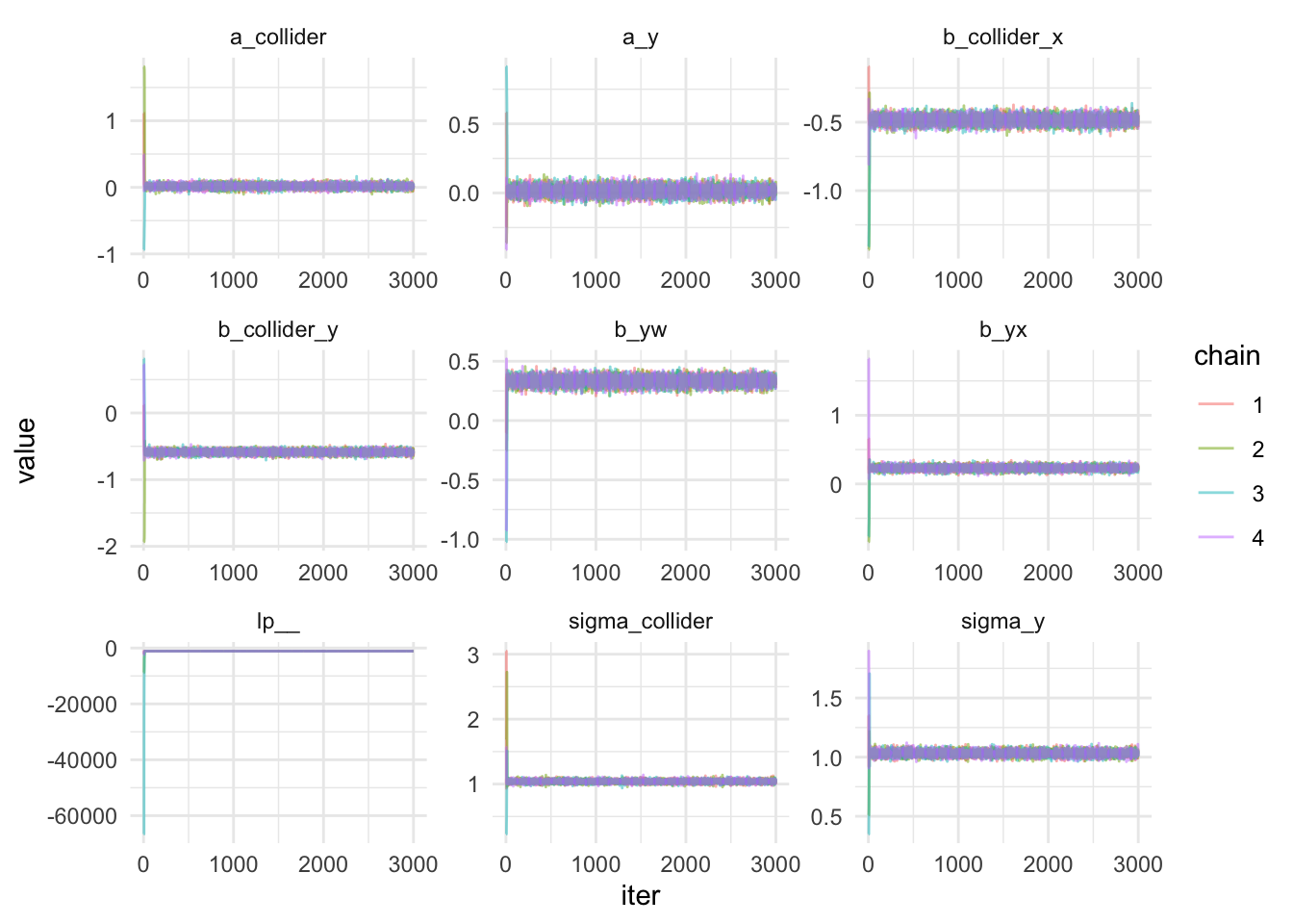
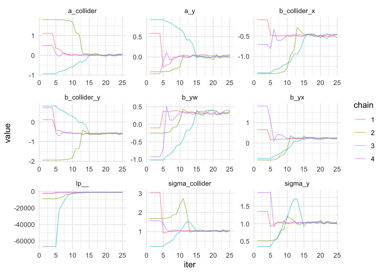
Notice that the iter is 3000 instead of 2000? That is because we included the warm up. Did you see how wide the parameters were the first few iterations and then they converge quite quickly, probably after 10 iterations. It’s hard to see that with the plot above. Let’s zoom in and filter out iters less than 25.
Zooming In Iterations < 25 🔍
mcmc_df |>
  filter(iter <= 25) |>
  ggplot(aes(x=iter,y=value,color=chain)) +
  geom_line(alpha=0.5) +
  facet_wrap(.~variable, scales = "free") +
  theme_minimal()

That’s pretty cool! The convergence occurred by iter 15!
Less Code to Visualize via Bayesplot
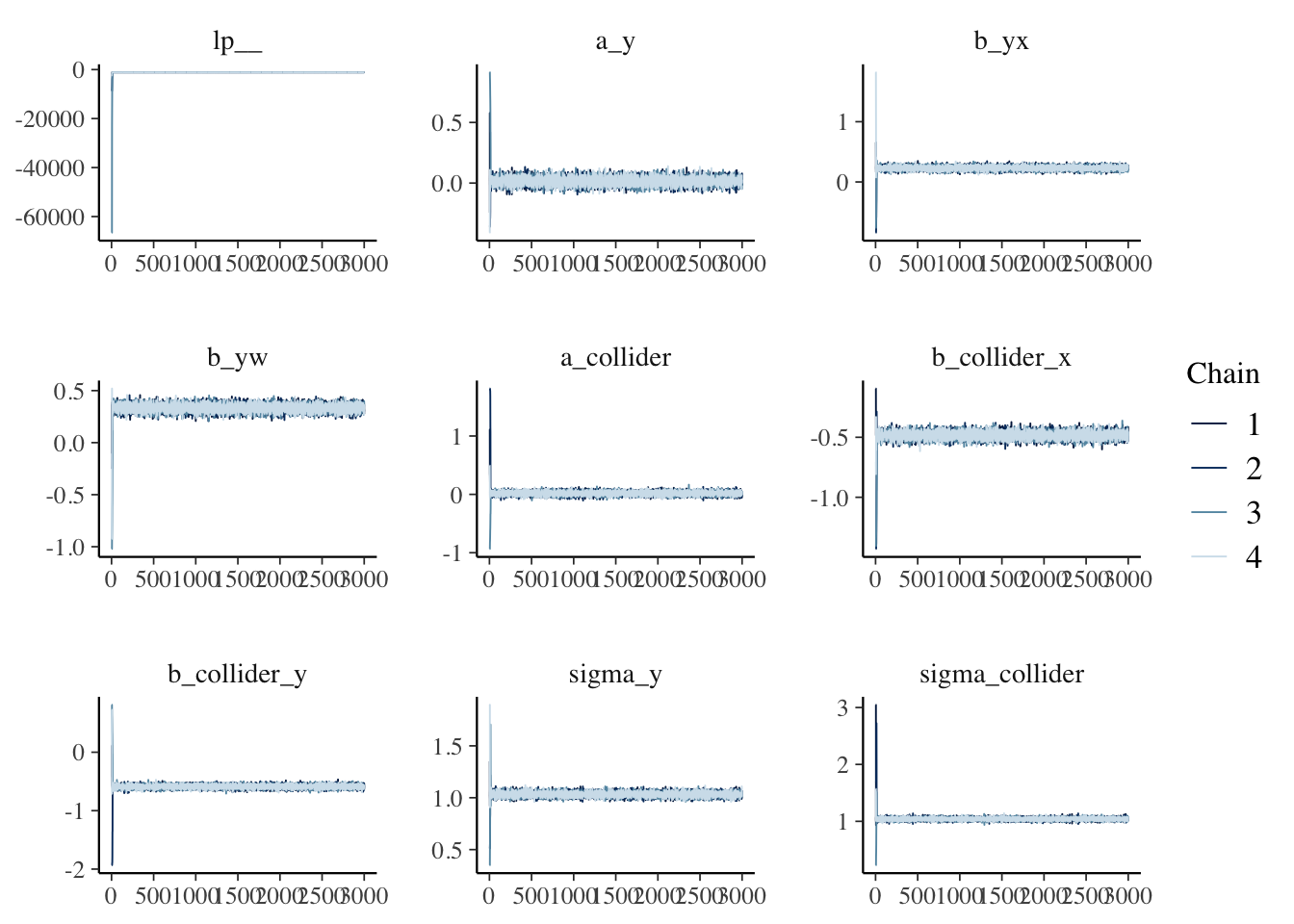
bayesplot::mcmc_trace(fit$draws(inc_warmup = T))

🤣 Much prettier than mine!
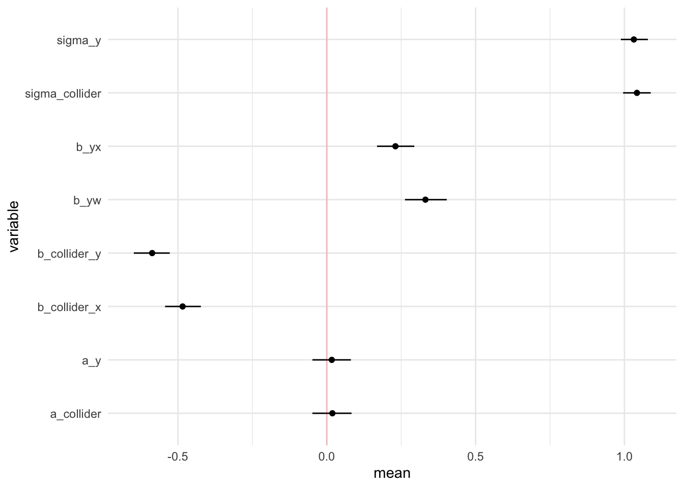
Esimates and Its 95% Credible Interval
mcmc_df |>
  group_by(variable) |>
  filter(variable != "lp__") |>
  summarize(mean = mean(value),
            lower = quantile(value, 0.025),
            upper = quantile(value, 0.975)) |>
  ggplot(aes(x=variable,y=mean,ymin=lower,ymax=upper)) +
  geom_point() +
  geom_linerange() +
  geom_hline(yintercept = 0, color = "red", alpha = 0.2) +
  coord_flip() +
  theme_minimal()

Things to Improve on / Learn
- Take a closer look on Rhat, ESS, and LP might be helpful diagnostics. Perhaps attempting to calculate all of these from scratch might lead to better understanding. I found an intersting article that explains lp__
- Looking at Logistic Regression next
- Applying Prior
- Then go back to the very question I have, how to apply this if I know the prior, sensitivity and specificty of a test. How to use Stan to calculate posterior.
- Explore the other Stan blocks (e.g., data generation, function etc.)
- Get a little more familiar with parameters and hyperparameters. A good tip is to read from bottom up, equation -> parameter -> hyperparameter.
Acknowledgement 🙏
A big thank-you to Alec Wong for helping me understand the basics of Bayesian statistics and MCMC. This guy is truly a genius! He has the ability to explain things clearly, even at my beginner level, which is quite impressive. Another person I’d like to thank is Jose Cañadas. If it weren’t for his inspirational comments about using ‘full luxury Bayes’ on one of my blog posts, I might not have revisited Bayesian statistics so quickly. Now, I understand some of the code he was trying to use with the rethinking package. Last but not least, I want to acknowledge LLM for being my personal tutor!
Lessons Learnt
- Learnt how to estimate LR coefficient with
cmdstanr - Learnt how to write out data, parameter, and model blocks in Stan
- Learnt about Rhat (wants it close to 1 and <1.05), ESS (>100), MCMC chains
- Learnt how to extract the posterior and visualize them
If you like this article:
- please feel free to send me a comment or visit my other blogs
- please feel free to follow me on twitter, GitHub or Mastodon
- if you would like collaborate please feel free to contact me
- Posted on:
- September 19, 2023
- Length:
- 9 minute read, 1826 words